Week 7 - Simulation of a 1D Supersonic nozzle flow simulation using Macormack Method

AIM:-

Simulation of a 1D Supersonic nozzle flow simulation using Macormack Method.

OBJECTIVE:-

In this challenge you are going to simulate the isentropic flow through a quasi 1D subsonic-supersonic nozzle. You will derive both the conservation and non-conservation forms of the governing equations and sovle them using the MacCormack's technique. You need to determine the steady-state temperature distribution for the flow-field variables and investigate the difference between the two forms of governing equations by comparing their solutions.

You need to show the following plots inside your report
1. Steady-state distribution of primitive variables inside the nozzle
2. Time-wise variation of the primitive variables
3. Variation of Mass flow rate distribution inside the nozzle at different time steps during the time-marching process
4. Comparison of Normalized mass flow rate distributions of both forms

THEORY:-

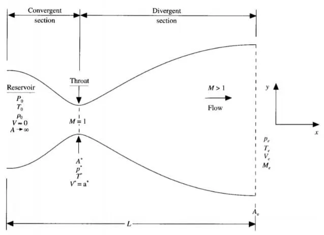
Consider Isentropic flow through a convergent-divergent nozzle. The flow at the inlet of the nozzle comes from the reservoir. The cross-section area of the reservoir is very large and hence velocity is very small(i.e v = 0 m/s at the inlet). The flow is locally subsonic in the convergent section of the nozzle, Sonic at the throat, and Supersonic at the divergent section. The 1D convergent-divergent nozzle is shown below,

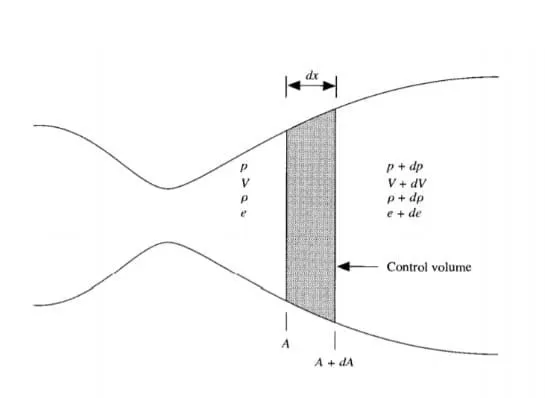
Let us consider a small control volume near the throat of the nozzle as shown below,

Assume that at a given section, the cross-section area is A, and the flow properties are uniform across the section. Hence, although the area of the nozzle changes as a function of distance along the nozzle, X, and therefore in reality the flow field is two-dimensional (the flow varies in the two-dimensional x-y space), We make the assumption that the flow properties vary only with X; this is tantamount to assuming uniform flow properties across any given cross-section. Such flow is defined as a Quasi-one-dimensional flow.

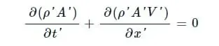
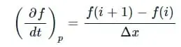
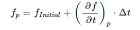
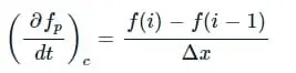
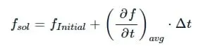
Governing Equations are represented in terms of PDE for both forms in order to use the Time Marching solution for the problem. The continuity, momentum, and energy governing equations (in terms of non-dimensional variables) for this quasi-one-dimensional steady isentropic flow can be expressed respectively as:

Non-Conservative form:-

1:- Continuity equation,

2:- Momentum equation:-

3:- Energy equation:-

Conservative Form:-

1:- Continuity equation:-

2:- Momentum equation:-

3:- Enegry equation:-

Maccormack Method:-

In this method we split time marching into predictor and corrector phase:

1:- Initial condition:-

The initial conditions of the profile for all the flow field variables which are velocity, density, and temperature have to be determined. these are guess values but should be specified with more awarness of the problem.

2:- Predictor step:-

In this step performed forward differencing for the space terms,

3:- Solution update :-

With the predictor values, the initial solutions are updated,

4:- Corrector step:-

In this step performed backward differencing for the space terms,

5:- Average derivative:-

Find the average for predictor and corrector steps,

6:- Final solution update:-

Final solution of the flow field variables for the first step,

SOLUTION:-

In this program there are 3 section:

1. Main program of 1D Supersonic nozzle

2. Non-conservative form

3. Conservative form

Main program:-

clear all

close all

clc

%INPUTS

%Number of grid points

n = 31;

gamma = 1.4;

x = linspace(0,3,n);

dx = x(2) - x(1);

%Number of time step

nt = 1400;

%Courant Number

C = 0.5;

%Function of Non-conservative

tic;

[Mass_flow_rate_NC, Pressure_NC, Mach_number_NC, rho_NC, v_NC, T_NC, rho_throat_NC, v_throat_NC, T_throat_NC, Mass_flow_rate_throat_NC, Pressure_throat_NC, Mach_number_throat_NC] = Non_conservative_form(x, dx, n, gamma, nt, C);

Time_elapsed_NC = toc;

fprintf('Time Elasped for Non Conservative form: %0.4f', Time_elapsed_NC);

hold on

%Plot

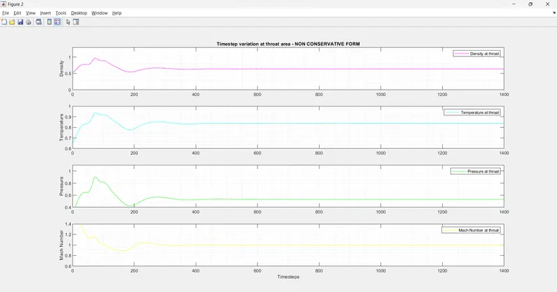
%Timestep variation of properties at throat area in Non-Conservative form

figure(2)

%Density

subplot(4,1,1)

plot(linspace(1,nt,nt),rho_throat_NC,'color','m')

ylabel('Density')

legend({'Density at throat'});

axis([0 1400 0 1.3]);

grid minor;

title('Timestep variation at throat area - NON CONSERVATIVE FORM')

%Temperature

subplot(4,1,2)

plot(linspace(1,nt,nt),T_throat_NC,'color','c')

ylabel('Temperature')

legend({'Temperature at throat'});

axis([0 1400 0.6 1]);

grid minor;

%Pressure

subplot(4,1,3)

plot(linspace(1,nt,nt),Pressure_throat_NC,'color','g')

ylabel('Pressure')

legend({'Pressure at throat'});

axis([0 1400 0.4 1.1]);

grid minor

%Mach Number

subplot(4,1,4)

plot(linspace(1,nt,nt),Mach_number_throat_NC,'color','y')

xlabel('Timesteps')

ylabel('Mach Number')

legend({'Mach Number at throat'});

axis([0 1400 0.6 1.4]);

grid minor;

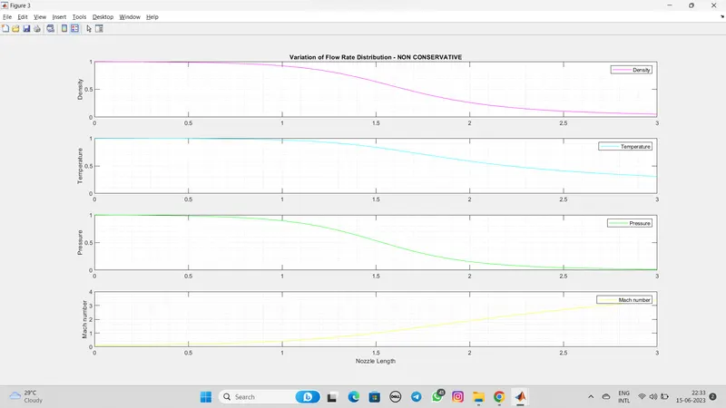
%Steady state simulation for primitve values for Non-Conservative form

figure(3);

%Density

subplot(4,1,1);

plot(x,rho_NC,'color','m')

ylabel('Density')

legend({'Density'});

axis([0 3 0 1])

grid minor;

title('Variation of Flow Rate Distribution - NON CONSERVATIVE')

%Temperature

subplot(4,1,2);

plot(x,T_NC,'color','c')

ylabel('Temperature')

legend({'Temperature'});

axis([0 3 0 1])

grid minor;

%Pressure

subplot(4,1,3);

plot(x,Pressure_NC,'color','g')

ylabel('Pressure')

legend({'Pressure'});

axis([0 3 0 1])

grid minor;

%Mach number

subplot(4,1,4);

plot(x,Mach_number_NC,'color','y')

xlabel('Nozzle Length')

ylabel('Mach number')

legend({'Mach number'});

axis([0 3 0 4])

grid minor;

%Function of conservative

tic;

[Mass_flow_rate_C, Pressure_C, Mach_number_C, rho_C, v_C, T_C, rho_throat_C, v_throat_C, T_throat_C, Mass_flow_rate_throat_C, Pressure_throat_C, Mach_number_throat_C] = Conservative_form(x, dx, n, gamma, nt, C);

Time_elasped_C = toc;

fprintf('Time Elasped for Conservative form: %0.4f', Time_elasped_C);

%Plot

%Timestep variation of properties at throat area in Conservative form

figure(5)

%Density

subplot(4,1,1)

plot(rho_throat_C,'color','m')

ylabel('Density')

legend({'Density at throat'});

axis([0 1400 0 1]);

grid minor;

title('Timestep variation at throat area - CONSERVATIVE FORM')

%Temperature

subplot(4,1,2)

plot(T_throat_C,'color','c')

ylabel('Temperature')

legend({'Temperature at throat'});

axis([0 1400 0.6 1]);

grid minor;

%Pressure

subplot(4,1,3)

plot(Pressure_throat_C,'color','g')

ylabel('Pressure')

legend({'Pressure at throat'});

axis([0 1400 0.2 0.8]);

grid minor

%Mach Number

subplot(4,1,4)

plot(Mach_number_throat_C,'color','y')

xlabel('Timesteps')

ylabel('Mach Number')

legend({'Mach Number at throat'});

axis([0 1400 0.6 1.4]);

grid minor;

%Steady state simulation for primitve values for Non Conservative form

figure(6);

%Density

subplot(4,1,1);

plot(x,rho_C,'color','m')

ylabel('Density')

legend({'Density'});

axis([0 3 0 1])

grid minor;

title('Variation of Flow Rate Distribution - CONSERVATIVE FORM')

%Temperature

subplot(4,1,2);

plot(x,T_C,'color','c')

ylabel('Temperature')

legend({'Temperature'});

axis([0 3 0 1])

grid minor;

%Pressure

subplot(4,1,3);

plot(x,Pressure_C,'color','g')

ylabel('Pressure')

legend({'Pressure'});

axis([0 3 0 1])

grid minor;

%Mach number

subplot(4,1,4);

plot(x,Mach_number_C,'color','y')

xlabel('Nozzle Length')

ylabel('Mach number')

legend({'Mach number'});

axis([0 3 0 4])

grid minor;

%Comparison plot

figure(7)

hold on

plot(x,Mass_flow_rate_NC,'r','linewidth',1.25)

hold on;

plot(x,Mass_flow_rate_C,'b','linewidth',1.25)

hold on;

grid on

legend('Non Conservative','Conservative');

xlabel('Length of the Domain')

ylabel('Mass Flow Rate')

title('Comparison of Normalized Mass Flow Rate of both forms')

EXPLANATIONS:-

• Program start with clear all,close all,clc wich is used to new start without previous value.
• First inputs parameters for the variables like x,dx,n,gamma,nt and C.
• tic command used for calculate the time elasped between the function.
• Then generate the plot for Time variation at throat area of both form,variation of flow distribution,comparision of normalized mass flow rate.
• All plot is computed as subplot of Density,Temperature,Pressure,Mach number etc.

NON-CONSERVITE FORM:-

%Function for Non-Conservative form

function [Mass_flow_rate_NC, Pressure_NC, Mach_number_NC, rho_NC, v_NC, T_NC, rho_throat_NC, v_throat_NC, T_throat_NC, Mass_flow_rate_throat_NC, Pressure_throat_NC, Mach_number_throat_NC] = Non_conservative_form(x, dx, n, gamma, nt, C)

%Intial boundary conditions

rho_NC = 1 - 0.3146*x;

T_NC = 1 - 0.2341*x;

v_NC = (0.1 + 1.09*x).*T_NC.^0.5;

%Area & Throat profiles

a = 1 + 2.2*(x - 1.5).^2;

throat = find(a==1);

%Outer Time Loop

for k = 1:nt

%Time-step control

dt = min(C.*dx./(sqrt(T_NC) + v_NC));

rho_old = rho_NC;

T_old = T_NC;

v_old = v_NC;

%Predictor Method

for j = 2:n-1

dv_dx = (v_NC(j + 1) - v_NC(j))/dx;

drho_dx = (rho_NC(j + 1) - rho_NC(j))/dx;

dT_dx = (T_NC(j + 1) - T_NC(j))/dx;

dlog_a_dx = (log(a(j + 1)) - log(a(j)))/dx;

%Continuity Equation

drho_dt_P(j) = -rho_NC(j)*dv_dx - rho_NC(j)*v_NC(j)*dlog_a_dx - v_NC(j)*drho_dx;

%Momentum Equation

dv_dt_P(j) = -v_NC(j)*dv_dx - (1/gamma)*(dT_dx + (T_NC(j)*drho_dx/rho_NC(j)));

%Energy Equation

dT_dt_P(j) = -v_NC(j)*dT_dx - (gamma - 1)*T_NC(j)*(dv_dx + v_NC(j)*dlog_a_dx);

%Solution Update

rho_NC(j) = rho_NC(j) + drho_dt_P(j)*dt;

v_NC(j) = v_NC(j) + dv_dt_P(j)*dt;

T_NC(j) = T_NC(j) + dT_dt_P(j)*dt;

end

%Corrector Method

for j = 2:n-1

dv_dx = (v_NC(j) - v_NC(j - 1))/dx;

drho_dx = (rho_NC(j) - rho_NC(j - 1))/dx;

dT_dx = (T_NC(j) - T_NC(j - 1))/dx;

dlog_a_dx = (log(a(j)) - log(a(j - 1)))/dx;

%Continuity Equation

drho_dt_C(j) = - rho_NC(j)*dv_dx - rho_NC(j)*v_NC(j)*dlog_a_dx - v_NC(j)*drho_dx;

%Momentum Equation

dv_dt_C(j) = - v_NC(j)*dv_dx - (1/gamma)*(dT_dx + (T_NC(j)*drho_dx/rho_NC(j)));

%Energy Equation

dT_dt_C(j) = - v_NC(j)*dT_dx - (gamma - 1)*T_NC(j)*(dv_dx + v_NC(j)*dlog_a_dx);

end

%Compute Average time

drho_dt = 0.5.*(drho_dt_P + drho_dt_C);

dv_dt = 0.5.*(dv_dt_P + dv_dt_C);

dT_dt = 0.5.*(dT_dt_P + dT_dt_C);

%Solution

for i = 2:n-1

rho_NC(i) = rho_old(i) + drho_dt(i)*dt;

v_NC(i) = v_old(i) + dv_dt(i)*dt;

T_NC(i) = T_old(i) + dT_dt(i)*dt;

end

%Boundary Conditions

%Inlet

rho_NC(1) = 1;

v_NC(1) = 2*v_NC(2) - v_NC(3);

T_NC(1) = 1;

%Outlet

rho_NC(n) = 2*rho_NC(n-1) - rho_NC(n - 2);

v_NC(n) = 2*v_NC(n - 1) - v_NC(n - 2);

T_NC(n) = 2*T_NC(n - 1) - T_NC(n - 2);

%Defining Mass flow rate, Pressure and Mach number

Mass_flow_rate_NC = rho_NC.*a.*v_NC;

Pressure_NC = rho_NC.*T_NC;

Mach_number_NC = (v_NC./sqrt(T_NC));

%Calculating Variables at throat section

rho_throat_NC(k) = rho_NC(throat);

T_throat_NC(k) = T_NC(throat);

v_throat_NC(k) = v_NC(throat);

Mass_flow_rate_throat_NC(k) = Mass_flow_rate_NC(throat);

Pressure_throat_NC(k) = Pressure_NC(throat);

Mach_number_throat_NC(k) = Mach_number_NC(throat);

%Plot

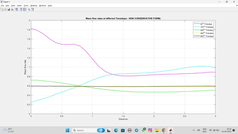
%Comparison of non-dimensional Mass flow rates at different time steps

figure(1);

if k == 50

plot(x, Mass_flow_rate_NC, 'm', 'linewidth', 1.25);

hold on

elseif k == 100

plot(x, Mass_flow_rate_NC, 'c', 'linewidth', 1.25);

hold on

elseif k == 200

plot(x, Mass_flow_rate_NC, 'g', 'linewidth', 1.25);

hold on

elseif k == 400

plot(x, Mass_flow_rate_NC, 'y', 'linewidth', 1.25);

hold on

elseif k == 800

plot(x, Mass_flow_rate_NC, 'k', 'linewidth', 1.25);

hold on

end

%Labelling

title('Mass flow rates at different Timesteps - NON CONSERVATIVE FORM)')

xlabel('Distance')

ylabel('Mass flow rate')

legend({'50^t^h Timestep','100^t^h Timestep','200^t^h Timestep','400^t^h Timestep','800^t^h Timestep'})

axis([0 3 0 2])

grid on

end

end

EXPLANATION:-

• In this programe we can calculate the values of Mass flow rate,Pressure,Mach number,Density,Velocity,Temperature,Density at throat,Velocity at throat,Temperature at throat,Mass floe rate at throat,Pressure at throat,Mach number at throat.
• Then calculate boundary conditions of density,Pressure,Temperature.
• Then find the valuse of area of throat,time loop.
• Calculate predictor and corrector method.

CONSERVITE FORM:-

%Function for Conservative form

function [Mass_flow_rate_C, Pressure_C, Mach_number_C, rho_C, v_C, T_C, rho_throat_C, v_throat_C, T_throat_C, Mass_flow_rate_throat_C, Pressure_throat_C, Mach_number_throat_C] = Conservative_form(x, dx, n, gamma, nt, C)

%Determining Initial profile of Density and Temperature

for i = 1:n

if (x(i) >= 0 && x(i) <= 0.5)

rho_C(i) = 1;

T_C(i) = 1;

elseif (x(i) >= 0.5 && x(i) <= 1.5)

rho_C(i) = 1 - 0.366*(x(i) - 0.5);

T_C(i) = 1 - 0.167*(x(i) - 0.5);

elseif (x(i) >= 1.5 && x(i) <= 3)

rho_C(i) = 0.634 - 0.3879*(x(i) - 1.5);

T_C(i) = 0.833 - 0.3507*(x(i) - 1.5);

end

end

%Area & Throat profiles

a = 1 + 2.2*(x - 1.5).^2;

throat = find(a==1);

%Initial profile fot Velocity and Pressure

v_C = 0.59./(rho_C.*a);

Pressure_C = rho_C.*T_C;

%Calculate the Initial Solution Vectors(U)

U1 = rho_C.*a;

U2 = rho_C.*a.*v_C;

U3 = rho_C.*a.*(T_C./(gamma - 1)) + ((gamma/2).*v_C.^2);

%Outer Time Loop

for k =1:nt

%Time-step control

dt = min(C.*dx./(sqrt(T_C) + v_C));

%Saving a copy of Old Values

U1_old = U1;

U2_old = U2;

U3_old = U3;

%Calculating the Flux vector(F)

F1 = U2;

F2 = ((U2.^2)./U1) + ((gamma - 1)/gamma)*(U3 - (gamma/2)*((U2.^2)./U1));

F3 = ((gamma*U2.*U3)./U1) - (gamma*(gamma - 1)*((U2.^3)./(2*U1.^2)));

%Predictor Method

for j = 2:n-1

%Calculating the Source term(J)

J2(j) = (1/gamma)*rho_C(j)*T_C(j)*((a(j + 1) - a(j))/dx);

%Continuity Equation

dU1_dt_P(j) = -((F1(j + 1) - F1(j))/dx);

%Momentum Equation

dU2_dt_P(j) = -((F2(j + 1) - F2(j))/dx) + J2(j);

%Energy Equation

dU3_dt_P(j) = -((F3(j + 1) - F3(j))/dx);

%Updating New values

U1(j) = U1(j) + dU1_dt_P(j)*dt;

U2(j) = U2(j) + dU2_dt_P(j)*dt;

U3(j) = U3(j) + dU3_dt_P(j)*dt;

end

%Updating Flux vectors

F1 = U2;

F2 = ((U2.^2)./U1) + ((gamma - 1)/gamma)*(U3 - ((gamma*0.5*(U2.^2))./(U1)));

F3 = ((gamma*U2.U3)./U1) - ((gamma*0.5*(gamma - 1)*(U2.^3))./(U1.^2));

%Corrector Method

for j = 2:n-1

%Updating the Source term(J)

J2(j) = (1/gamma)*rho_C(j)*T_C(j)*((a(j) - a(j - 1))/dx);

%Simplifying the Equation's spatial terms

dU1_dt_C(j) = -((F1(j) - F1(j - 1))/dx);

dU2_dt_C(j) = -((F2(j) - F2(j - 1))/dx) + J2(j);

dU3_dt_C(j) = -((F3(j) - F3(j - 1))/dx);

end

%Compute Average Time derivative

dU1_dt = 0.5*(dU1_dt_P + dU1_dt_C);

dU2_dt = 0.5*(dU2_dt_P + dU2_dt_C);

dU3_dt = 0.5*(dU3_dt_P + dU3_dt_C);

%Final Solution Update

for i = 2:n-1

U1(i) = U1_old(i) + dU1_dt(i)*dt;

U2(i) = U2_old(i) + dU2_dt(i)*dt;

U3(i) = U3_old(i) + dU3_dt(i)*dt;

end

%Boundary Conditions

%Inlet

U1(1) = rho_C(1)*a(1);

U2(1) = 2*U2(2) - U2(3);

v_C(1) = U2(1)./U1(1);

U3(1) = U1(1)*((T_C(1)/(gamma - 1)) + ((gamma/2)*(v_C(1)).^2));

%Outlet

U1(n) = 2*U1(n - 1) - U1(n - 2);

U2(n) = 2*U2(n - 1) - U2(n - 2);

U3(n) = 2*U3(n - 1) - U3(n - 2);

%Final Primitive value update

rho_C = U1./a;

v_C = U2./U1;

T_C = (gamma - 1)*((U3./U1 - (gamma/2)*(v_C).^2));

%Defining Mass flow rate, Pressure and Mach number

Mass_flow_rate_C = rho_C.*a.*v_C;

Pressure_C = rho_C.*T_C;

Mach_number_C = (v_C./sqrt(T_C));

%Calculating Variables at throat section

rho_throat_C(k) = rho_C(throat);

T_throat_C(k) = T_C(throat);

v_throat_C(k) = v_C(throat);

Mass_flow_rate_throat_C(k) = Mass_flow_rate_C(throat);

Pressure_throat_C(k) = Pressure_C(throat);

Mach_number_throat_C(k) = Mach_number_C(throat);

%plot

%Comparison of non-dimensional Mass flow rates at different time steps

figure(4)

if k == 50

plot(x, Mass_flow_rate_C, 'm', 'linewidth', 1.25);

hold on

elseif k == 100

plot(x, Mass_flow_rate_C, 'c', 'linewidth', 1.25);

hold on

elseif k == 200

plot(x, Mass_flow_rate_C, 'g', 'linewidth', 1.25);

hold on

elseif k == 400

plot(x, Mass_flow_rate_C, 'y', 'linewidth', 1.25);

hold on

elseif k == 800

plot(x, Mass_flow_rate_C, 'k', 'linewidth', 1.25);

hold on

end

%Labelling

title('Mass flow rates at different Timesteps - CONSERVATIVE FORM')

xlabel('Distance')

ylabel('Mass flow rate')

legend({'50^t^h Timestep','100^t^h Timestep','200^t^h Timestep','400^t^h Timestep','800^t^h Timestep'})

axis([0 3 0.4 1])

grid on

end

end

EXPLANATION:-

• In this also find the value of Mass flow rate,Pressure,Mach number,Density,Velocity,Temperature,Density at throat,Velocity at throat,Temperature at throat,Mass floe rate at throat,Pressure at throat,Mach number at throat to determine initial profile of Density and Temperature for loop.
• In this code to simplify and avoid errors equations is splitted into solution vector(U),flux vector(F)and source term(J).
• After that calculate Outer time loop is calculate for loop to all grid points for various loop.
• The Predictor and corrector method are assigned within the for loop individually calculate.
• Then boundary condition are applied for the calculate the mass flow rate,mach number and pressure and also calculate the value of throat section.
• After that generate the plot.

OUTPUTS:-

CONCLUSION:-

• From all results we can obsorved the Conservative form is converges slightly faster than the Non-conservative form.
• The conservation from produced a stable solution along the simulation.
• Both forms are dependable in calculation the solution.