Challenge

Project 2 - Rankine cycle Simulator

AApurva Patel31 Jan 2023

AIM:-

To create a MATLAB Program that calculate that state points of the Rankine Cycle.

OBJECTIVE:-

To create a Rankine Cycle Simulator using MATLAB.
To determine its state points including Net work output & Back work ratio.
Plot its T-S and h-S diagram from the given data.
Explain its working.

THEORY:-

The Rankine Cycle is an idealized thermodynamic cycle describing the process by which certain heat engines,such as steam turbine or reciprocating steam engines, allow mechanical work to be extracted from a fluid as it moves between a heat source and heat sink.

LAYOUT OF THE RANKINE CYCLE:-

Turbine
Condenser
Pump
Boiler

In the Rankine cycle, the following processes take place:-

PROCESS 1-2 :-

The dry saturated vapour expands through a turbine, generating power. This decreases the temperature and pressure of the vapour and some condensation may occure.

Process 1-2 is isentropic expansion in the turbine.

PROCESS 2-3 :-

The wet vapour then enters a condenser, Where it is condensed at a constant pressure to become a saturated liquid. Process 2-3 is constant pressure heat rejection or isobaric heat rejection by the condenser.

PROCESS 3-4 :-

The working fluid is pumped from low to high pressure. As the fluid is a liquid at this stage, the pump requires little input energy. Process 3-4 is isentropic compression in the pump.

PROCESS 4-1 :-

The high-pressure liquid enters a boiler, Where it is heated at constant pressure by an external heat source to become a dry saturated vapour. Process 4-1 is constant pressure heat addition or isobaric heat transfer addition or isobaric heat transfer by the boiler.

GIVEN INPUTS :-

Turbine inlet pressure = 30 bars

Turbine inlet temperature = 400 C

Turbine outlet pressure or Condenser inlet pressure = 0.05 bars.

MATLAB CODE :-

The MATLAB code of Rankine Cycle as below,

% Program to calculate the state point of the Rankine cycle simulator

clear all

close all

clc

% Step-1

fprintf('Rankine Cycle Simulator n n')

fprintf('Process 1-2 is Isentropic Expansion in the Turbine n ')

fprintf('Process 2-3 is Isobaric Heat Rejection by the condenser n ')

fprintf('Process 3-4 is Isentropic Compression in the Pump n ')

fprintf('Process 4-1 is Isobaric Heat Transfer by the Boiler n ')

% Step-2 : Input variables

P1 = input('Enter the pressure at the Turbine inlet (in bar) : ');

T1 = input('Enter the temperature at the turbine inlet (in Degree Celcius) : ');

P2 = input('Enter the pressure at the Condenser (in bar) : ');

t = linspace(0,400,500);

disp('')

% Step-3 : Calculation of state point of the Rankine Cycle

% At state point 1

H1 = XSteam('h_pT',P1,T1);

S1 = XSteam('s_pT',P1,T1);

hl1 = XSteam('hl_p',P1);

hg1 = XSteam('hV_p',P1);

sl1 = XSteam('sL_p',P1);

sg1 = XSteam('sV_p',P1);

Tsat1 = XSteam('Tsat_p',P1);

% At state point 2

S2 = S1;

sl2 = XSteam('sL_p',P2);

sg2 = XSteam('sV_p',P2);

d = (S1 - sl2)./(sg2 - sl2);

hl2 = XSteam('hL_p',P2);

hg2 = XSteam('hV_p',P2);

H2 = hl2 + (d.*(hg2 - hl2));

T2 = XSteam('T_ph',P2, H2);

Tsat2 = XSteam('Tsat_p',P2);

% At the state point 3

P3 = P2;

S3 = sl2;

H3 = hl2;

T3 = T2;

% At the state point 4

P4 = P1;

S4 = S3;

H4 = XSteam('h_ps', P4, S4);

T4 = XSteam ('T_ps', P4, S4);

% Step IV : Calculate Work Done & Thermal Efficiency

% Work done by the turbine

Wt = H1 - H2;

% Work done by the pump

Wp = H4 - H3;

% Net Work done

Wnet = Wt - Wp;

% Thermal Efficiency

thermal_efficiency = (1 - ((H2 - H3)./(H1 - H4))).*100;

% Back Work Ratio

back_work_ratio = Wp./Wt;

% Specific Steam Conductivity

SSC = 3600./Wt;

% Step V : Plotting T-S Diagram for Rankine Cycle

figure(1), clf

hold on

% Saturation Curve

% 'r' indicates Marker's red color & '.' indicates its shape

for i = 1 : length(t)

plot(XSteam('sL_T',t(i)),t(i),'r.')

plot(XSteam('sV_T',t(i)),t(i),'r.')

end

% Cycle

plot([S1 S2], [T1 T2], 'LineWidth',3)

text(S1,T1+10, '1', 'FontSize',11)

if d > 1

T3 = Tsat2;

plot([S2 sg2 S3 S4], [T2 Tsat2 T3 T4], 'LineWidth', 3)

T2 = Tsat2;

text(S2,T2-10, '2', 'FontSize',11)

text(S3,T3-10, '3', 'FontSize',11)

else

plot([S2 S3 S4], [T2 T3 T4], 'LineWidth', 3)

text(S2,T2-10, '2', 'FontSize',11)

text(S3,T3-10, '3', 'FontSize',11)

end

n = linspace(T1, T2, 500);

for i = 1 : length(n)

plot(XSteam('s_pT',P1,n(i)),n(i),'.','Linewidth',3,'Color','b')

end

axis([0 10 0 450])

plot([sl1 sg1], [Tsat1 Tsat1], 'LineWidth',3)

text(sl1,Tsat1-10, '4', 'FontSize',11)

xlabel('Entrophy (kJ/kg K)')

ylabel('Temperature (K)')

title('T-S Diagram for Rankine Cycle')

grid on

% Step VI : Plotting h-S Diagram for Rankine Cycle

figure(2), clf

hold on

% Saturation Curve

for i = 1 : length(t)

plot(XSteam('sL_T',t(i)), XSteam('hL_T', t(i)),"Color",'r','Marker','.')

plot(XSteam('sV_T',t(i)), XSteam('hV_T', t(i)),"Color",'r','Marker','.')

end

% Process Cycle

plot([S1 S2 S3 S4 S1], [H1 H2 H3 H4 H1],'LineWidth',3, 'Color','b')

text(S1,H1+80,'1','FontSize', 15)

text(S2,H2-80,'2','FontSize', 15)

text(S3,H3-60,'3','FontSize', 15)

text(S4,H4+180,'4','FontSize', 15)

xlabel('Entrophy (kJ/kg K)');

ylabel('Enthalphy (kJ/kg)');

title('h-S Diagram for Rankine Cycle');

grid on

% Step VII : Displaying Results in the command window

fprintf('Final Results n n')

% At State Point 1

disp('At State Point 1: ')

fprintf('P1 = %.2f Bar n',P1)

fprintf('T1 = %.2f Deg Celcius n',T1)

fprintf('H1 = %.2f kJ/kg n',H1)

fprintf('S1 = %.2f kJ/kg K n',S1)

disp(' ')

% At State Point 2

disp('At State Point 2: ')

fprintf('P2 = %.2f Bar n',P2)

fprintf('T2 = %.2f Deg Celcius n',T2)

fprintf('H2 = %.2f kJ/kg n',H2)

fprintf('S2 = %.2f kJ/kg K n',S2)

disp(' ')

% At State Point 3

disp('At State Point 3: ')

fprintf('P3 = %.2f Bar n',P3)

fprintf('T3 = %.2f Deg Celcius n',T3)

fprintf('H3 = %.2f kJ/kg n',H3)

fprintf('S3 = %.2f kJ/kg K n',S3)

disp(' ')

% At State Point 4

disp('At State Point 4: ')

fprintf('P4 = %.2f Bar n',P4)

fprintf('T4 = %.2f Deg Celcius n',T4)

fprintf('H4 = %.2f kJ/kg n',H4)

fprintf('S4 = %.2f kJ/kg K n',S4)

disp(' ')

fprintf('Work done by the turbine = %.2f kJ/kg n', Wt)

fprintf('Work done by the pump = %.2f kJ/kg n', Wp)

fprintf('Net work done = %.2f kJ/kg n', Wnet)

fprintf('Thermal Efficiency = %.2f % n', thermal_efficiency)

fprintf('nBack work ratio = %f', back_work_ratio)

fprintf('nSpecific Steam Conductivity = %.2f kg/kWh n', SSC)

MATLAB CODE EXPLANATION :-

Program start with the writing comments
Then add clear all, close all and clc.
After that put Inputs like Turbine inlet pressure, Turbine inlet temperature and Turbine outlet pressure which take from Xsteam file.
Defining the spacific heat for the values for liquid and vapour using the Xsteam table
Then define the saturation temperature Tsat using Xsteam.
After that properties specific enthalpy and entropy at state ,1,2,3,4 using the Xsteam table
Then calculate the turbine work,pump work, net work, thermal efficiency, specific fuel consumpation.
Then plot the saturation dome along with the rankine cycle process curve in T-S diagram.
Then plot the saturation dome along with the rankine cycle process curves in H-S diagram.
After that display the result in command window.

ERROR FACING :-

Facing the error while program as below,

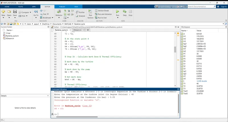
The error occure if we do not properly define the correct variable, It can be corrected by writing in proper way.

RESULT:-

From above results, we can see that thr given problem statement is executed by calculating the thermodynamic properties and plotting the curves of all the species.

Specific enthalpy and entropy values are calculated for different states are calculated for different states and T-S and H-S diagram are plotted.

Result of code as below,

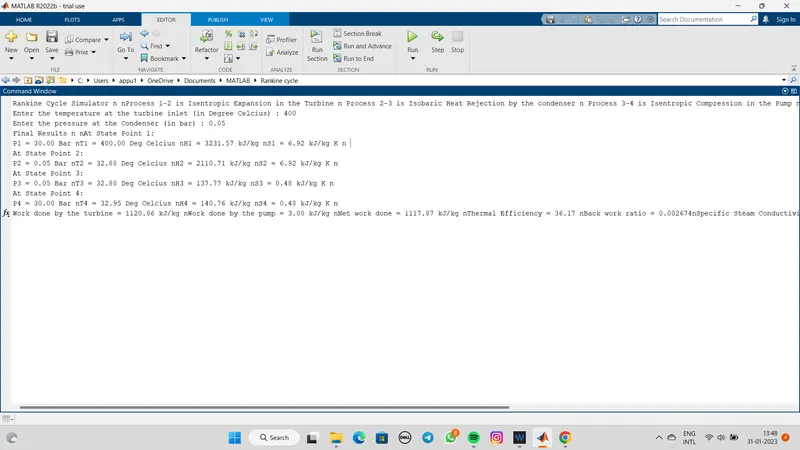
1-Net work done = 1117.87 kJ/kg

2-Thermal Efficiency = 36.17%

3-Back work ratio = 0.002674

Project 2 - Rankine cycle Simulator

Ship work like this
in your own course.

Talk to a career counsellor

Ship work like thisin your own course.

Talk to a career counsellor

Ship work like this
in your own course.