Week 1- Mixing Tee

AIM:-

To create a two case of the mixing tee. One of them is longer than the other. Our job is to set steady-state sumylations to compare the mixing the 36celsius and and the cold inlet is at 19celsius. Also use the k-eplison and k-omega SST model for the first case based and your judjemtent use the more suitable model for futhther cases.

CASE:-1

• Short mixing tee with a hot inlet velocity of 3m/s.
• Momentum ratio of 2, 4.

CASE:-2

• Long mixing tee with a hot inlet velocity of 3m/s.
• Momentum ratio of 2, 4.

• Momentum ratio = velocity at cold inlet / velocity at hot inlet

  In a table, compare the following values from the 2 cases.

  1. Cell count
  2. Average outlet temperature
  3. Number of iterations for convergence

Expected results:

1. Velocity and temperature contour plots on the cut planes along and across the pipe.
2. Velocity and temperature line plots along and across the length of the pipe.
3. Perform Mesh independent study for any one case.
4. Discuss the effect of length and momentum ratio on results.
5. For each simulation, you need to show the convergence plot.

INTRODUCTIONS:-

Mixing tee are commonly used in the petrochemical industry to blend two fluid stream with different physical and chemical properties. Temperature fluctuations in the metal may cause thermal fatigue in the pressure boundary pipes. If theew is through-wall cracking,the fluid may leak, causing a fire and other hazards. As a result it is critical to ensure to ensure that temperature difference are kept to a minium so that the pipe system can withstand them. Redesigning the pipe system system so that the momentum ratio of the fluid streams is advantageous for mixing is one option as is installing sytems that protect the pressure boundary piping to improve mixing and prevent temperature swings.

THEORY:-

In this tee junctions simulation the same fluid is fixed at varied temperatures and inlet velocities through two perpendicular inlet pipes to calculate temperature change. The simulation is repeated twice with the only variable being the geometry length. Further more for each example we will simulate for momentum ratio of 2 and 4. The K- and K- SST models are emplodyed for the first example and the more approptite model is untilised for subsequent cause based on the decision. The K-Epsilon model is best suitable for the flow away from the wall such as free surface flow. The K-Omega model is best suited for near wall-flow region where an unfavourable pressure gradient develops.

Geometry:- using the Space claim the volume of fluid which is gonna be studied is extracted by selecting the edges of the model

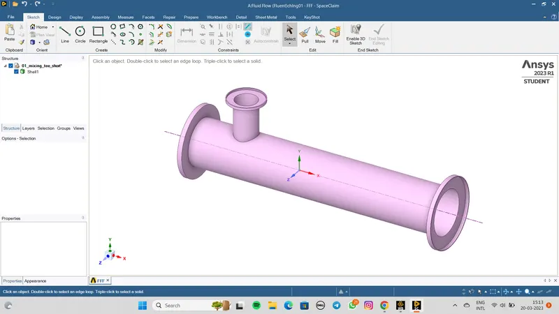
After Edges preperation:-

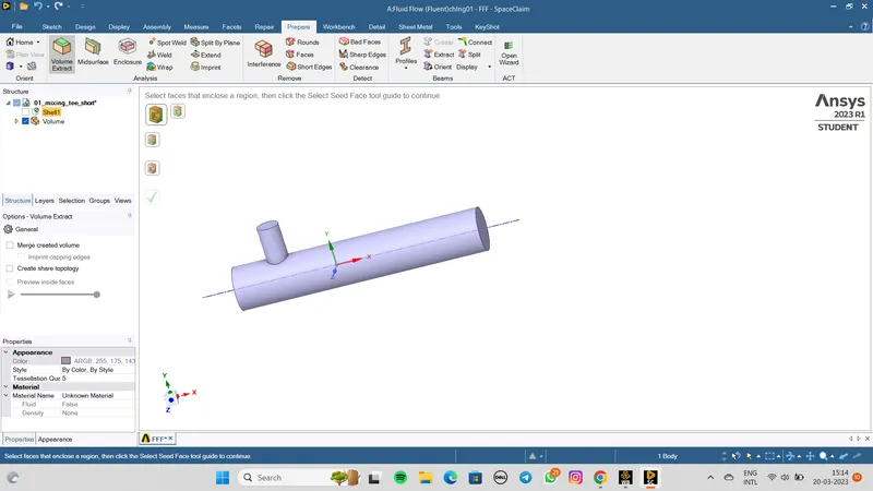
After this Mesh process will be start:-

Mesh: Mesh generated over the entire geometry, then boundaries of the geometry is given names. The whole geometry is cut in half to seen the mesh within the geometry.

Inlet X: Inlet along the x direction.
Inlet Y: Inlet along the Y direction.
Outlet: Outlet along the x direction.
Wall: The entire boundary of the extratced volume is selected

After Add the name half cut with the section plane and get a graph as per below,

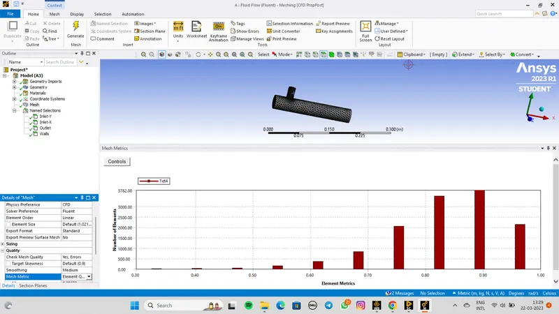
After Mesh process Setup and solution steps where the add some values like,

Case_1A:- Short Tee

Momentum Ratio = 2
Inlet Temperature along the x axis = 36*C, flow velocity=3m/s
Inlet Temperature along the x axis = 19*C, flow velocity=6m/s
K – epsilon, realizable, wall standard function

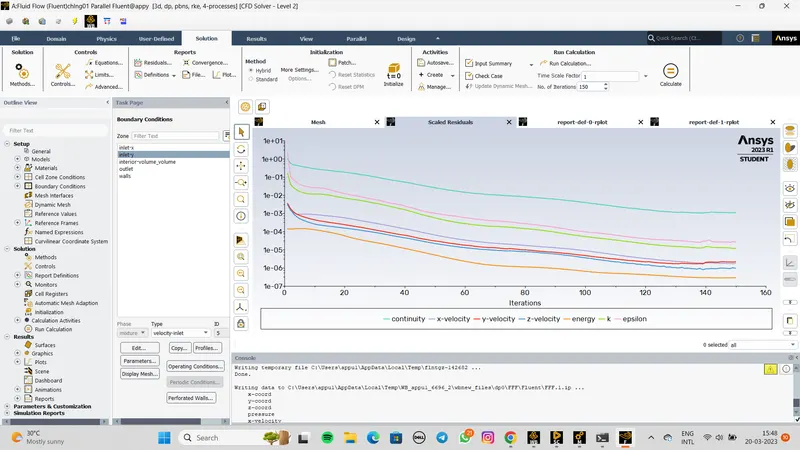
Then the calculate the programe and we get graph as below,

Residual:-

Standard Deviation:-

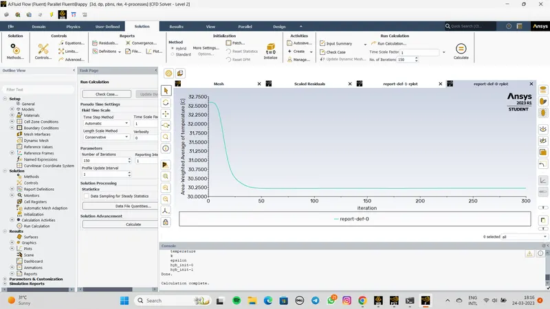
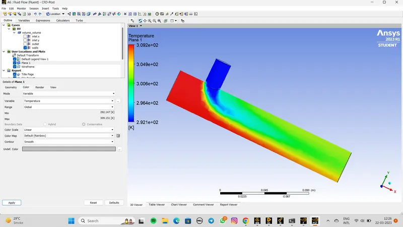
After this process we get Result and also get graph for Temperature and Velocity as below,

Temperature:-

Velocity:-

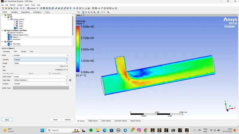
Now, there are 2nd case K-Omega

Geometry and Meshing process are same as K-Epsilon.

Case_1B:- Short Tee

Momentum Ratio = 4
Inlet Temperature along the x axis = 36*C, flow velocity=3m/s
Inlet Temperature along the x axis = 19*C, flow velocity=6m/s
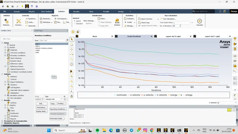
K – omega, SST

Then the calculate the programe and we get graph as below,

Residual:-

Standard Deviation:-

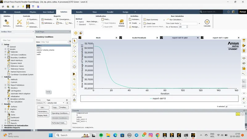
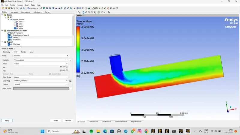
After this process we get Result and also get graph for Temperature and Velocity as below,

Temperature:-

Velocity:-

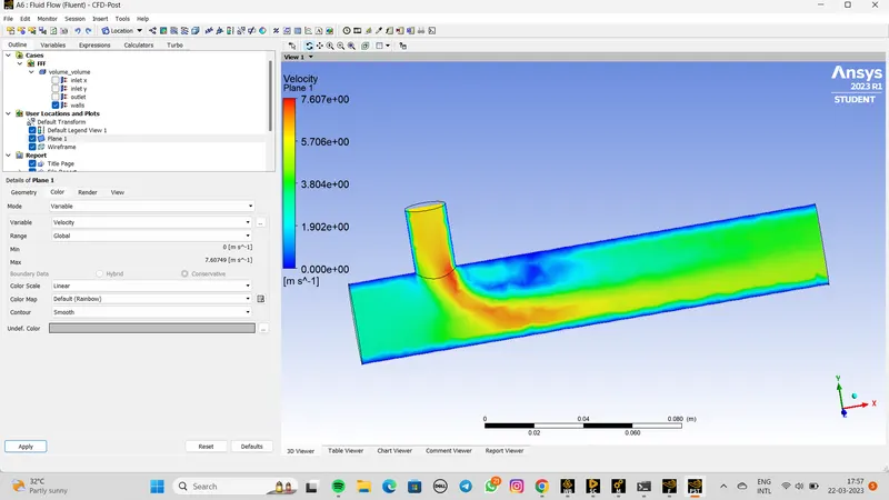
• By comparing the above couture’s we can say that K-w SST model is extracting model turbulence effect compare with k-epsilon model.
• We can say that for getting converge solutions k-w SST model is taking more time compare with k-epsilon model.
• Finally, we can say that we can use k-w SST turbulence model for further simulations.

Case of Long Tee:-

Geometry:- Value Extracted

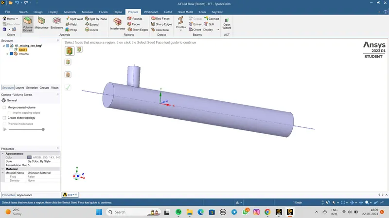
Meshing Process:-

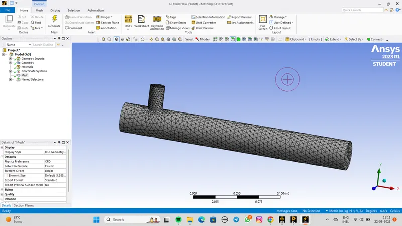
Plot Process

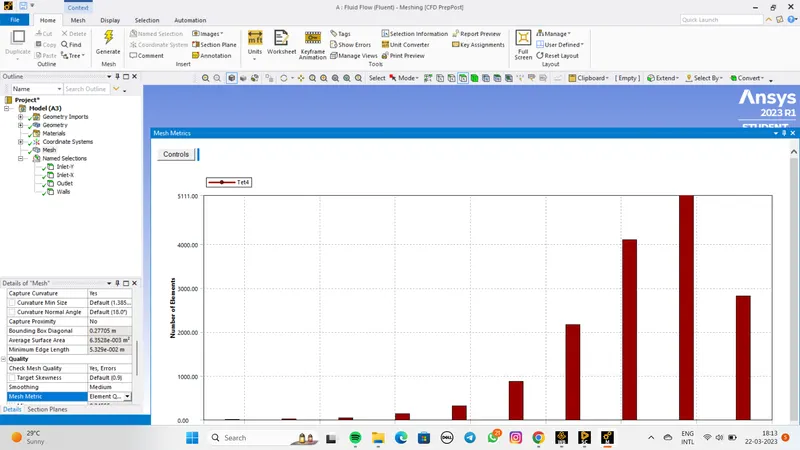
After that the calculate the programe and we get graph as below,

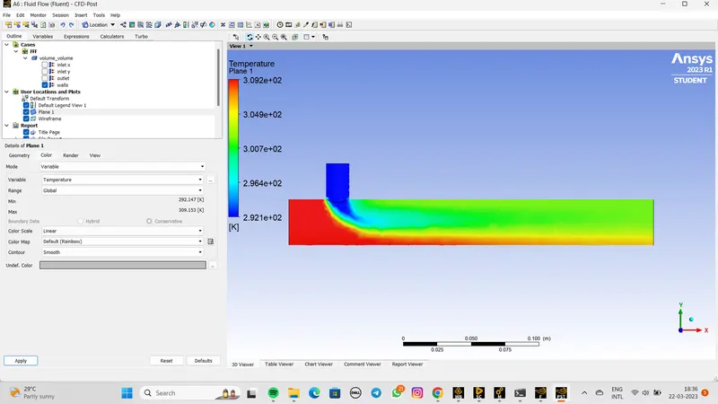
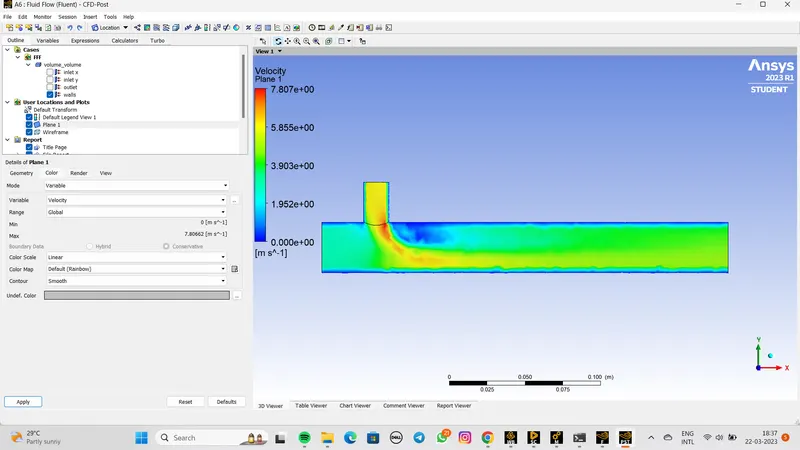
Case_2A:- Long Tee

Momentum Ratio = 2
Inlet Temperature along the x axis = 36*C, flow velocity=3m/s
Inlet Temperature along the x axis = 19*C, flow velocity=6m/s
K – epsilon, realizable, wall standard function

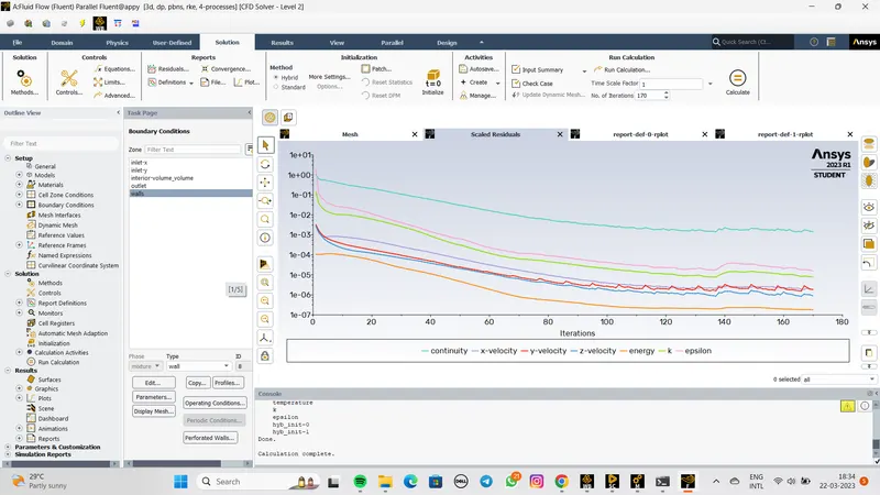
After Calculation we get the graph and results as below,

Residual:

Standard Deviation:

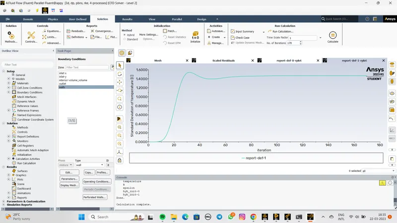
After this process we get Result and also get graph for Temperature and Velocity as below,

Temperature:-

velocity:-

Now the program for 2nd case of Long tee

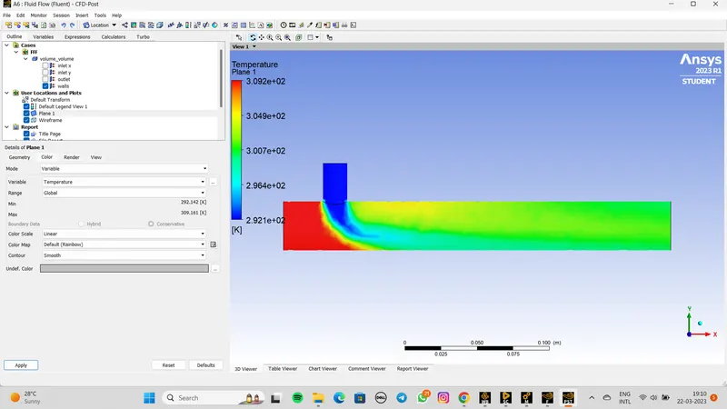
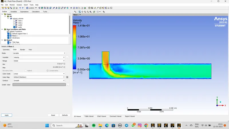
Case_2B:- Long Tee

Momentum Ratio = 4
Inlet Temperature along the x axis = 36*C, flow velocity=3m/s
Inlet Temperature along the x axis = 19*C, flow velocity=12m/s
K – epsilon, realizable, wall standard function

Geometry and meshing process are Similar to long tee with 1st case for long tee.

Temperature:-

Velocity:-

CONCULATION:-

• To get better mixing at outlet, high velocity is preferred so momentum ratio of 4 has better mixing results at outlet.
• As the length of the mixing tee increases, the mixing time is more before it exits from the outlet. Thus the long mixing tee has better mixing characteristics.
• As the mesh size is coarser, the number of iterations required to converge to final result is less. But as the mesh size gets finer, the number of iterations for convergence increases since there are more number of cells to perform simulation.