Week 5.1 - Mid term project - Solving the steady and unsteady 2D heat conduction problem

AIM:-

To solve the steady and unsteady 2D heat condution problem using the iterative method.

OBJECTIVE:-

• To perform steady-state analysis & unsteady state analysis.
• To understand the different iterative techniques used to solve the steady and unsteady 2D heat conduction problem.

GIVEN DATA:-

Top Boundary = 600 K

Bottom Boundary = 900 K

Left Boundary = 400 K

Right Boundary = 800 K

SOLVING METHODS:-

• Jacobi
• Gauss-seidel
• Successive over-relaxation

THEORY:-

• Heat conduction is defined as the process by which heat is transferred from the hotter end to the colder end of the object.
• The heat conduction equation is a second-order partial differential equation that describes the distribution of heat energy in a given body over time.

2D Heat Conduction:-

∂^2T/∂t^2+a(∂^2T/∂x^2+∂y^2)=0

STEADY-STATE 2D HEAT CONDUCTION:-

In a steady-state heat transfer the heat flow rate remains constant at any point in time. Steady-state heat transfer can be described in terms of the temperature as the variable the temperature of the system remains constant over time in steady-state heat transfer after thermal equillibrium is attained.

∂^2T/∂x^2+∂^2T/∂y^2=0

Transient state 2D Heat Conduction:-

Transient heat transfer can also be called unsteady-state heat transfer. This type of heat transfer only exists for a short duration of time. In transient heat transfers, the heat energy transferred through the medium is not constant. The heat flow rate keeps changing, and the cause of the varying rates of heat transfer can be either fluctuating temperature differences over the medium or changes in properties of the medium.

In the physical world, heat transfer starts as transient and then reaches a steady state until thermal equilibrium is reached.

∂2T∂t2+α(∂2T∂x2+∂2T∂y2)=0

INTERATIVE SOLVER:

1. JACOBI METHOD:-In this method the temperature (n+1)interation is found using old values of the temperature defined at nth iterations.Using the approximation obtained iteration procedure is continued untill the desired accurancy of the solution is obtained.

2. GAUSS - SEIDEL METHOD:- In this type of iterative solver, the temperature at n+1 iterations uses values of n+1 iterations that have already been computed. In this way, old approximated values are overwritten with new approximate values for the iterations performed. Unlike Jacobi, Gauss seidel requires one storage vector which can be overwritten with each computation.

3. Successive over-relaxation method:- In this type of iterative solver relaxation factor is used which helps in increasing the convergence rate.

MATLAB CODE:-

1:-

EXPLANATION:-

• First of all program start with clear all, close all, clc.
• After that input given data as bellow
• L is for domain length is 1

OUTPUT:-

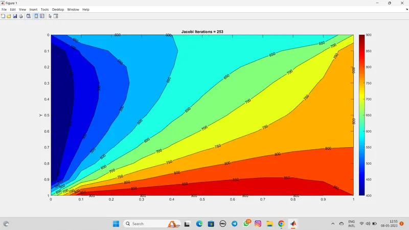
1. Jacobi:-

For the uniformaly space grid please enter the number of grid points: 11

Enter an option for type of solver you would like use: 1

TIME_Taken =

53.2683

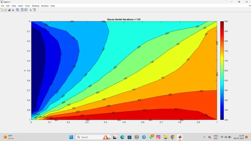
2. GAUSS SEIDEL:-

For the uniformaly space grid please enter the number of grid points: 11

Enter an option for type of solver you would like use: 2

TIME_Taken =

27.3742

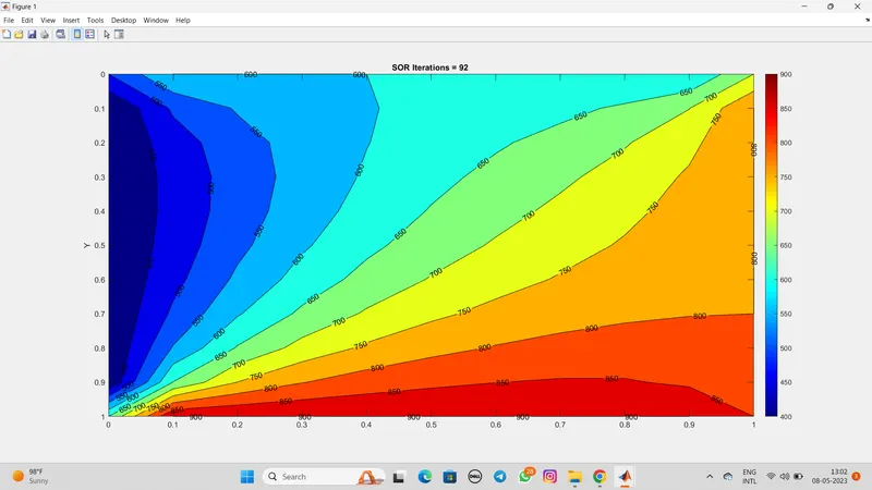
3.SOR:-

For the uniformaly space grid please enter the number of grid points: 11

Enter an option for type of solver you would like use: 3

TIME_Taken =

20.9876

MATLAB CODE:-

2:-EXPLICIT METHOD

clear all

close all

clc

% EXPLICIT METHOD

L=1;

nx=input('For the uniformly space grid please enter the number of grid points:');

ny=nx;

x=linspace(0,L,nx);

y=linspace(L,0,ny);

dx=L/(nx-1);

dy=L/(ny-1);

dt=0.001;

%t=0.1;

%nt=t/dt;

error=9e9;

tol=1e-4;

T_L=400;

T_R=800;

T_T=600;

T_B=900;

T=298*ones(nx,ny);

T(1,:)=T_B;

T(end,:)=T_T;

T(:,1)=T_L;

T(:,end)=T_R;

T(1,1)=(900+400)/2;

T(1,end)=(900+800)/2;

T(end,1)=(400+600)/2;

T(end,end)=(800+600)/2;

alpha=1.4; %Diffusivity

k1=alpha*dt/dx^2;

k2=alpha*dt/dy^2;

[X,Y]=meshgrid(x,y);

Told=T;

CFL=k1+k2 %To verify if the solution is stable within the limit CFL(x)+CFL(y)=0.5

unsteady_explicit_iter=1;

tic

for nt=1:1400

while(error>tol)

for i=2:nx-1

for j=2:ny-1

term1=Told(i-1,j)-2*Told(i,j)+Told(i+1,j);

term2=Told(i,j-1)-2*Told(i,j)+Told(i,j+1);

T(i,j)=Told(i,j)+k1*term1+k2*term2;

end

end

error=max(max(abs(Told-T)));

Told=T;

unsteady_explicit_iter=unsteady_explicit_iter+1;

figure(1)

[A,B]=contourf(X,Y,T);

set(gca,'YDIR','reverse')

colorbar

colormap(jet)

clabel(A,B);

text=sprintf('Unsteady Explicit Iterations = %d',unsteady_explicit_iter);

ylabel('Y')

title(text)

pause(0.03)

end

end

Time_Taken=toc

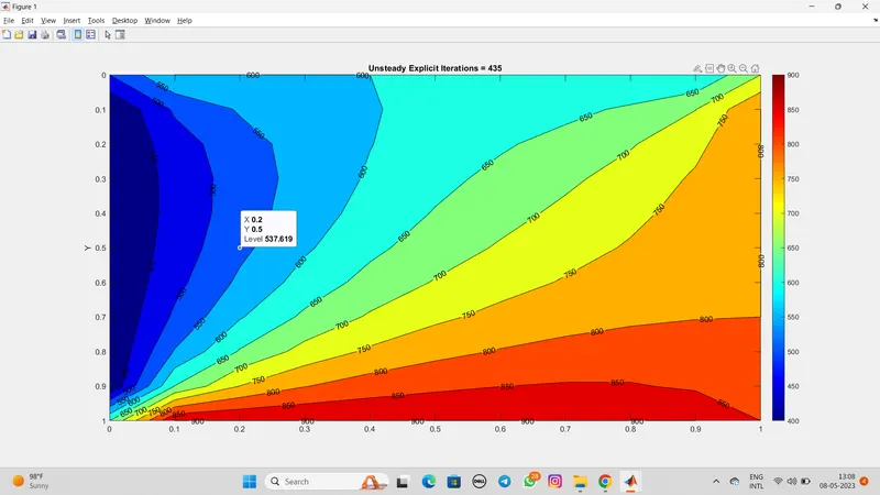
OUTPUT :-

For the uniformaly space grid please enter the number of grid points: 11

CFL =

0.2800

Time Taken =

116.2568

MATLAB CODE:-

3. IMPLICIT METHOD:-

clear all

close all

clc

% IMPLICIT METHOD

L=1;

nx=input('For the uniformly space grid please enter the number of grid points:');

ny=nx;

x=linspace(0,L,nx);

y=linspace(L,0,ny);

dx=1/(nx-1);

dy=1/(ny-1);

alpha=1.4;

dt=0.001;

%error=9e9

tol=1e-4;

T_L=400;

T_R=800;

T_T=600;

T_B=900;

T=298*ones(nx,ny);

T(1,:)=T_B;

T(end,:)=T_T;

T(:,1)=T_L;

T(:,end)=T_R;

T(1,1)=(900+400)/2;

T(1,end)=(900+800)/2;

T(end,1)=(400+600)/2;

T(end,end)=(800+600)/2;

k1=alpha*dt/dx^2;

k2=alpha*dt/dy^2;

CFL=k1+k2

Told=T;

T_prev_dt=T;

iter=1;

omega=1.1;

iterative_solver=input('1) Jacobi 2) Gauss Seidel 3) SOR \nEnter an option for the type of solver you would like to use: \n');

tic

for nt=1:1400

if iterative_solver==1

term1=(1+2*k1+2*k2)^(-1);

term2=k1*term1;

term3=k2*term1;

error=9e9;

while(error>tol)

for i=2:nx-1

for j=2:ny-1

H=(Told(i-1,j)+Told(i+1,j));

V=(Told(i,j-1)+Told(i,j+1));

T(i,j) = (T_prev_dt(i,j)*term1)+(H*term2)+(V*term3);

end

end

error=max(max(abs(Told-T)));

Told=T;

iter=iter+1;

end

end

if iterative_solver==2

term1=(1+2*k1+2*k2)^(-1);

term2=k1*term1;

term3=k2*term1;

error=9e9;

while(error>tol)

for i=2:nx-1

for j=2:ny-1

H=(T(i-1,j)+Told(i+1,j));

V=(T(i,j-1)+Told(i,j+1));

T(i,j) = (T_prev_dt(i,j)*term1)+(H*term2)+(V*term3);

end

end

error=max(max(abs(Told-T)));

Told=T;

iter=iter+1;

end

end

if iterative_solver==3

term1=(1+2*k1+2*k2)^(-1);

term2=k1*term1;

term3=k2*term1;

error=9e9;

while(error>tol)

for i=2:nx-1

for j=2:ny-1

H=(T(i-1,j)+Told(i+1,j));

V=(T(i,j-1)+Told(i,j+1));

T(i,j) = (1-omega)*Told(i,j)+omega*((T_prev_dt(i,j)*term1)+(H*term2)+(V*term3));

end

end

error=max(max(abs(Told-T)));

Told=T;

iter=iter+1;

end

end

T_prev_dt=T;

end

Time_Taken=toc

figure(1)

[P Q]=contourf(x,y,T);

set(gca,'YDIR','reverse')

colorbar;

colormap(jet);

clabel(P,Q);

text=sprintf('Implicit Iterations = %d',iter);

ylabel('Y')

title(text)

%pause(0.03)

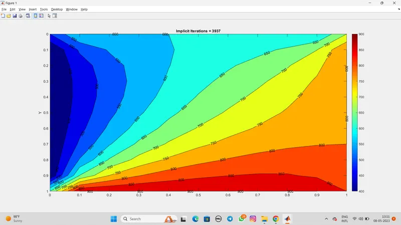
OUTPUT:-

1. JACOBI METHOD:-

For the uniformaly space grid please enter the number of grid points: 11

Enter an option for type of solver you would like use: 1

TIME_Taken =

0.0341

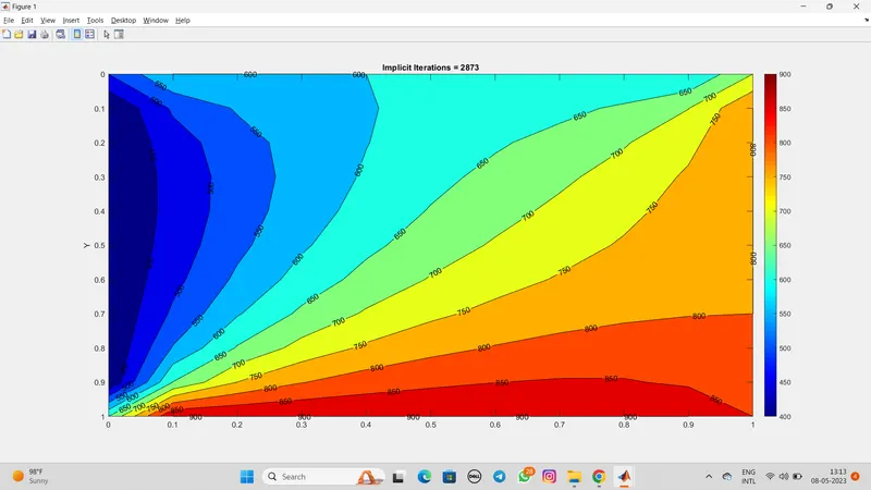
2. GAUSS SEIDEL METHOD:-

For the uniformaly space grid please enter the number of grid points: 11

Enter an option for type of solver you would like use: 2

TIME_Taken =

0.0290

3. SOR:-

For the uniformaly space grid please enter the number of grid points: 11

Enter an option for type of solver you would like use: 3

TIME_Taken =

0.0301

RESULT:-

• In steady state methods, there is no time loop and the results converge within a few interations, we include time loop for implicit methods and it runs for a large number iterations.
• Transient solver take a lot of time for computation as it is a function of both time and position when comparing to steady solver which is only a function of position.
• The SOR provide us the answer with less number of irerations and takes less time.

CONCLUSION:-

The 2D heat conduction equation was solved making use of iterative techniques.