Week 7 - Simulation of a 1D Supersonic nozzle flow simulation using Macormack Method

Title :- Simulation of the isentropic flow through a quasi 1D subsonic-supersonic nozzle using Macormack Method

Aim/Objectives :-

• To derive both the conservation and non-conservation forms of the governing equations for the quasi 1D subsonic-supersonic nozzle
• Solve the governing equations using the MacCormack's technique
• To determine the steady-state temperature distribution for the flow-field variables and investigate the difference between the two forms of governing equations (Conservative and Non-conservative) by comparing their solutions
• Plot the steady-state distribution of primitive variables inside the nozzle across the length of the nozzle
• To show the Mass flow rate distribution inside the nozzle at different time steps
• Perform grid/mesh independency test to see the effect of grid size on our solution
• Analyse and validate the results with CFD book by John Anderson textbook

Introduction :

In this quasi 1 dimensional subsonic-supersonic nozzle flow problem, we will consider the steady, isentropic flow through a convergent-divergent nozzle. The flow at the inlet to the nozzle comes from a reservoir where the pressure and temperature are denoted by po, and To, respectively. The velocity is very small (V `to` 0) at the inlet due to the large cross-sectional area of the eservior. Thus, po and To are the stagnation values, or total pressure and total temperature, respectively. The flow expands isentropically to supersonic speeds at the nozzle exit, where the exit pressure, temperature, velocity, and Mach number are denoted by Pe, Te, Ve, and Me, respectively.

The flow is locally subsonic (Mach number <1) in the convergent section of the nozzle, means at the convergent section local velocity of the fluid is less than the velocity of the sound at the same medium sonic at the throat (minimum area), and supersonic (maximum area at the divergent section. The sonic flow (M = 1) at the throat means that the local velocity at this location is equal to the local speed of sound. At the throat section we have denoted the area, pressure, temperature and velocity as `A^ast`,`p^ast`,`T^ast` and `V^ast = a^ast` respectively.

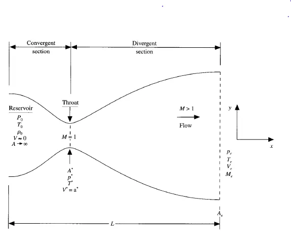
FIG. 1 Schematic diagram of subsonic-supersonic isentropic nozzle flow

We have assumed that, where the cross-sectional areais A, the properties of the flow are uniform means that the velocity of the flow is the same magnitude and dirction at every point in fluid. Althogh, the area of the nozzle changes with distance along the nozzle therefore in reality flow field is two dimensional. And we make the assumption that the flow properties vary only with x(length of nozzle). Such flow is called as quasi 1 dimensional flow.

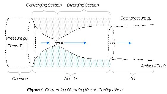
FIG. 2 Schematic diagram of subsonic-supersonic isentropic nozzle flow

What is quasi 1 dimensional flow : Quasi 1-D flows are very similar to 1 D flows. In quasi 1D flow we assume flow is compressible and steady. Tha gas behaves as an ideal gas and its property variations are assumed to be isentropic. Viscous effects are neglected. The solid boundaries are adiabatic means there is no heat tarnsfer takes place between system and surrounding. The main difference between the 1D and Quasi 1D flows is the cross-sectional area of the passage. In 1 D flows cross-sectional area is constant and only the flow variables vary with respect to x. For quasi 1D flows it is no longer constant, but is a function of the length of the nozzle (x location). The properties of the flow are assumed to be uniform across the passage and only vary in the x direction.

We will solve the nozzle flow problem using both non-conservative and conservative form of governing equations by helping of MacCormack's Technique.

Governing Equations for non-conservative form:

Continuity equation

`(delrho')/(delt')=-rho'(delV')/(delx')-rho'V'(del(lnA)')/(delx')-V'(delrho')/(delx')`

Momentum equation

`(delV')/(delt')=-V'((delV')/(delx'))-1/gamma((delT')/(delx')+(T')/(rho')(delrho')/(delx'))`

Energy equation

`(delT')/(delt')=-V'(delT')/(delx')-(gamma-1)T'[(delV')/(delx')+V'(del(lnA)')/(delx')]`

Governing Equations for conservative form:

Continuity equation

`(del(rho^'A^'))/(delt^')+(del(rho^'A^'v^'))/(delx^')=0`

Momentum equation

`(del(rho^'A^'v^'))/(delt^')+(del[rho^'A^'v^('^2)+1/gamma*p^'A^'])/(delx^')=1/gamma*p^'*(delA^')/(delx^')`

Energy equation

`(del[rho^'(e^'/(gamma-1)+gamma/2*v^('^2))*A^'])/(delt^')+(del[rho^'*(e^'/(gamma-1)+gamma/2*v^('^2))*v^'*A^'+p^'*A^'*v^'])/(delx^')=0`

Solution variables

`U1=-rho'A'`

`U2=rho'A'V'`

`U3=rho'A'((e')/(gamma-1)+(gamma)/2V'^2)`

Flux terms

F1 = U2

F2 = `(U2^2)/(U1)+(gamma-1)/gamma(U3-gamma/2(U2^2)/(U1))`

F3 = `gamma(U2U3)/(U1)-(gamma(gamma-1))/2(U2^3)/(U1^2)`

Source term in Momentum equation

J2 = `1/gammarho^'T^'(delA)/(delx)`

MacCormack's Technique:

Mackeromack method is a widely used discretization scheme for time marching approach of hyperbolic equation.MacCormack's Technique is a variant of Lax-Wendroff approach. It is much simpler in application. This is explicit finite difference technique. The results obtained from MacCormack's technique are satisfactory as it is second order accurate in both space and time.

Steps involved in MacCormack's method

• Predictor step (Replace the spatial derivatives with on the right hand side with forward differencing)
• Solution update
• Corrector step (Replace the spatial derivatives with on the right hand side with backward differencing)
• Determining the average of the time derivative
• Final solution update

Predictor Step

In predictor step we replace the spatial derivatives with on the right hand side with forward differencing. In order to get clear idea , if we consider continuity equation

`((del rho)/(delt))_(i,j)^t=-(rho_(i,j)^t.(u_(i+1,j)^t-u_(i,j)^t)/dx+u_(i,j)^t.(rho_(i+1,j)^t-rho_(i,j)^t)/dx)`

Here we can see that on right hand side we replace spatial derivatives with forward differencing.

Corrctor step

In corrector step , we first obtain a predicted value of the time derivative at time t+`Deltat` by subsituting the predictive values of rhp, u and v into the right side of the equation . Then , we replace the the spatial derivatives with backward differencing.

`((del rho)/(delt))_(i,j)^(t+Deltat)=-(rho_(i,j)^(t+Deltat).(u_(i,j)^(t+Deltat)-u_(i-1,j)^(t+Deltat))/dx+u_(i,j)^(t+Deltat).(rho_(i,j)^(t+Deltat)-rho_(i-1,j)^(t+Deltat))/dx)`

The average value is obtained from the average of predicted and corrector step.

`((delrho)/(delt))_(avg)=0.5[((delrho)/(delt))_(p)+((delrho)/(delt))_(c)]`he numerical solution is calculated as an average value.

Here p stands for predictor step and c for corrector step in MacCormack's method.

Main script file for nozzle flow problem

clear all
close all
clc

%Inputs
n = 31;
x = linspace(0,3,n);
dx = x(2)-x(1);
%Courant number
C = 0.5;
nt = 1400;
gamma = 1.4;


tic;
[rho_NC,t_NC,v_NC,a_NC,pressure_NC,rho_throat_NC,temp_throat_NC, pressure_throat_NC,mass_flow_NC,mass_flow_throat_NC,mass_flow_time_NC] = non_conservative_form(n,x,dx,gamma,nt,C);
Time_taken = toc;
fprintf('Time elapsed for non conservative form = %4.2f secondn', Time_taken);

tic;
[rho_C,t_C,p_C,v_C,a_C,rho_throat_C,temp_throat_C, pressure_throat_C,mass_flow_C,mass_flow_throat_C,mass_flow_time_C] = conservative_form(n,x,dx,gamma,nt,C);
Time_taken_conservative = toc;
fprintf('Time elapsed for conservative form = %4.2f secondn', Time_taken_conservative);


% Mass flow rate comparison between conservative and Non-conservative forms
figure(7)
plot(x,mass_flow_NC,'linewidth',1.5)
hold on
plot(x,mass_flow_C,'linewidth',1.5)
title('Mass flow rate comparison','FontSize',12)
xlabel('Distance along Nozzle (Non-Dimensional)');
ylabel('Mass flow rate-(Non-Dimensional)');
grid on
legend('Non-conservative','conservative')

Explanation of code :

• We are going to solve this 1 D quasi nozzle flow problem in both forms Non-conservations and conservations using Maccormick's technique.
• First of all as usual, clear all , close all and clc has used to clear the workspace variables, figure window and command window. Then , given the necessary inputs for this problem such as n, x, nt,gamma,etc..
• Next line , we have called the function to solve this problem with Non-conservation and Conservation governing equations. We have written two different function code for tha same.
• Also to calculate the amount of time taken to execute the solution, tic and toc has used.

Function code for Non-conservative form

function [rho_NC,t_NC,v_NC,a_NC,pressure_NC,rho_throat_NC,temp_throat_NC, pressure_throat_NC,mass_flow_NC,mass_flow_throat_NC,mass_flow_time_NC] = non_conservative_form(n,x,dx,gamma,nt,C)


%Calculate initial profiles
rho_NC = 1-0.31468*x;
t_NC = 1-0.2314*x; %t for temperature
v_NC = (0.1+1.09*x).*t_NC.^0.5;

%Area
a_NC = 1+2.2*(x-1.5).^2;
throat_loc_NC = find(a_NC==1);



%Outer time loop
for k = 1:nt

    dt_NC = min(C.*(dx./(sqrt(t_NC)+(v_NC))));


    rho_old_NC = rho_NC;
    v_old_NC = v_NC;
    t_old_NC = t_NC;

    %Predictor method
    for j = 2:n-1
        dvdx = (v_NC(j+1)-v_NC(j))/dx;
        drhodx = (rho_NC(j+1)-rho_NC(j))/dx;
        dtdx = (t_NC(j+1)-t_NC(j))/dx;
        dlogadx = (log(a_NC(j+1))-log(a_NC(j)))/dx;

        %Continuity equation
        drhodt_p(j) = -rho_NC(j)*dvdx-rho_NC(j)*v_NC(j)*dlogadx-v_NC(j)*drhodx;

        %Momentum equation
        dvdt_p(j) = -v_NC(j)*dvdx - (1/gamma)*(dtdx +(t_NC(j)/rho_NC(j))*drhodx);

        %Energy equation
        dtdt_p(j) = -v_NC(j)*dtdx-(gamma-1)*t_NC(j)*(dvdx+v_NC(j)*dlogadx);

        %Solution update
        rho_NC(j) = rho_NC(j)+drhodt_p(j)*dt_NC;
        v_NC(j) = v_NC(j)+dvdt_p(j)*dt_NC;
        t_NC(j) = t_NC(j)+dtdt_p(j)*dt_NC;

    end

    %Corrector method
    for j = 2:n-1
        dvdx = (v_NC(j)-v_NC(j-1))/dx;
        drhodx = (rho_NC(j)-rho_NC(j-1))/dx;
        dtdx = (t_NC(j)-t_NC(j-1))/dx;
        dlogadx = (log(a_NC(j))-log(a_NC(j-1)))/dx;

        %Continuity equation
        drhodt_c(j) = -rho_NC(j)*dvdx-rho_NC(j)*v_NC(j)*dlogadx-v_NC(j)*drhodx;

        %Momentum equation
        dvdt_c(j) = -v_NC(j)*dvdx - (1/gamma)*(dtdx +(t_NC(j)/rho_NC(j))*drhodx);

        %Energy equation
        dtdt_c(j) = -v_NC(j)*dtdx-(gamma-1)*t_NC(j)*(dvdx+v_NC(j)*dlogadx);


    end

    %Compute average time derivative to obtain the final solution
    drhodt = 0.5*(drhodt_p + drhodt_c);
    dvdt = 0.5*(dvdt_p + dvdt_c);
    dtdt = 0.5*(dtdt_p + dtdt_c);

    %Final solution update
    for i = 2:n-1

        rho_NC(i) = rho_old_NC(i) + drhodt(i)*dt_NC;
        v_NC(i) = v_old_NC(i) + dvdt(i)*dt_NC;
        t_NC(i) = t_old_NC(i) + dtdt(i)*dt_NC;
    end

    %Apply boundary condition manually
    %Inlet boundary condition
    v_NC(1) = 2*v_NC(2) - v_NC(3);

    %Outlet boundary condition
    rho_NC(n) = 2*rho_NC(n-1)-rho_NC(n-2);
    v_NC(n) = 2*v_NC(n-1)-v_NC(n-2);
    t_NC(n) = 2*t_NC(n-1)-t_NC(n-2);

    pressure_NC = rho_NC.*t_NC;
    mass_flow_NC=rho_NC.*a_NC.*v_NC;

    %Primitive variables at location throat

    pressure_throat_NC(k)=pressure_NC(throat_loc_NC);
    rho_throat_NC(k)=rho_NC(throat_loc_NC);
    temp_throat_NC(k)=t_NC(throat_loc_NC);
    Velocity_throat_NC(k)=v_NC(throat_loc_NC);
    mass_flow_throat_NC(k) = mass_flow_NC(throat_loc_NC);

    mass_flow_time_NC(k,:)  = mass_flow_NC;
    pressure_time_NC(k,:) = pressure_NC;



end


%Plotting of the primitive variables along the domain
figure (1)
subplot (4,1,1)
plot(x,v_NC./sqrt(t_NC),'LineWidth',1.5,'Color','r')
xlabel('x')
ylabel('Mach')
legend('Mach number')
title('Primitive variables along the length of nozzle -Non-Conservative Form','FontSize',12)

subplot (4,1,2)
plot(x,pressure_NC,'LineWidth',1.5,'Color','k')
xlabel('x')
ylabel('Pressure')
legend('Pressure')

subplot (4,1,3)
plot(x,rho_NC,'LineWidth',1.5,'Color','g')
xlabel('x')
ylabel('Density')
legend('Density')

subplot (4,1,4)
plot(x,t_NC,'LineWidth',1.5,'Color','b')
xlabel('x')
ylabel('Temperature')
legend('Temperature')

%Variation of primitive variables at throat location with time steps
figure(2)
subplot(4,1,1)
plot(1:nt,rho_throat_NC,'LineWidth',1.5,'Color','r')
xlabel('Time step')
ylabel('Density throat')
legend('Density at throat')
title('Time-step Variation of primitive variables at throat area- Non conservative form','FontSize',12)

subplot(4,1,2)
plot(1:nt,temp_throat_NC,'LineWidth',1.5,'Color','k')
xlabel('Time step')
ylabel('Temp throat')
legend('Temperature at throat')

subplot(4,1,3)
plot(1:nt,pressure_throat_NC,'LineWidth',1.5,'Color','g')
xlabel('Time step')
ylabel('Pressure throat')
legend('Pressure at throat')

subplot(4,1,4)
plot(1:nt,Velocity_throat_NC./sqrt(temp_throat_NC),'LineWidth',1.5,'Color','b')
xlabel('Time step')
ylabel('Mach')
legend('Mach number at throat')

%Plotting Mass flow rate at different time steps along the domain
figure(3)
plot(x,mass_flow_time_NC(50,:),'LineWidth',1.5,'Color','g')
xlabel('Legth of the domain')
ylabel('Mass flow rate')
title('Mass flow rate at different time steps- Non-conservative Form','FontSize',12)
hold on
plot(x,mass_flow_time_NC(100,:),'LineWidth',1.5,'Color','r')
plot(x,mass_flow_time_NC(150,:),'LineWidth',1.5,'Color','k')
plot(x,mass_flow_time_NC(200,:),'LineWidth',1.5,'Color','m')
plot(x,mass_flow_time_NC(700,:),'LineWidth',1.5,'Color','b')
grid on
legend('50','100','150','200','700')




end

Explanation of code :

• Calculated the initial profile and area of the domain. And then we have find the location of the throat area where Area = 1.
• Outer time loop has started and it will execute till number of time steps whatever we have given. Within this time loop , using Maccormick's method we have calculated the governing equations for predictor and then for corrector method from node number 2 to (n-1) because we know the boundary conditions.
• Within this time loop calculation of the value of time step size has done.
• After the corrector method, we have taken the average of time derivative of Predictor and Corrector step in order to obtain the final solution.
• Next, we have updated the final solution for the last time and assigned the inlet and outlet boundary conditions.
• After that, calculated the flow filed variables throghout the nozzle and also at the throat location.
• And then outer time loop comes to an end and from the next line plotting has been started.

Function code for conservative form

function [rho_C,t_C,p_C,v_C,a_C,rho_throat_C,temp_throat_C, pressure_throat_C,mass_flow_C,mass_flow_throat_C,mass_flow_time_C] = conservative_form(n,x,dx,gamma,nt,C)


%Calculate initial profiles
for i = 1:n

    if (x(i) >= 0 && x(i) <= 0.5)
        rho_C(i) = 1;
        t_C(i) = 1;
    elseif (x(i) > 0.5 && x(i) <= 1.5)
        rho_C(i) = 1 - (0.366*(x(i) - 0.5));
        t_C(i) = 1 - (0.167*(x(i) - 0.5));
    elseif (x(i) > 1.5 && x(i) <= 3.5)
        rho_C(i) = 0.634 - (0.3879*(x(i) - 1.5));
        t_C(i) = 0.833 - (0.3507*(x(i) - 1.5));
    end

end


%Area & Throat profiles
a_C = 1 + (2.2*(x - 1.5).^2);
throat_loc_C = find(a_C==1);

%Initial profile fot Velocity and Pressure
v_C = 0.59./(rho_C.*a_C);
p_C = rho_C.*t_C;

%Calculate the Initial Solution Vectors(U)
U1 = rho_C.*a_C;
U2 = rho_C.*a_C.*v_C;
U3 = rho_C.*a_C.*(t_C./(gamma - 1)) + ((gamma/2).*v_C.^2);

%-------Macromack Method----%
% ----Conservation Equation------------%

%Outer time loop
for k = 1:nt

    dt_C = min(C.*dx./(sqrt(t_C)+v_C)); %Calculating the minimum time steps size value

    U1_old = U1;
    U2_old = U2;
    U3_old = U3;

    %Compute of flux vectors F1,F2,F3
    F1 = U2;
    F2 = ((U2.^2)./U1)+((gamma-1)/gamma)*(U3-(gamma/2)*((U2.^2)./U1));
    F3 = ((gamma*U2.*U3)./U1)- (gamma*(gamma-1)*((U2.^3)./(2*U1.^2)));

    %Predictor step
    for j = 2:n-1
        %Source terms in momentum equation
        j2(j) = (1/gamma)*rho_C(j)*t_C(j)*((a_C(j+1)-a_C(j))/dx);

        % Continuity, Momentum & Energy Equations
        dU1_dt_p(j) = -((F1(j+1)-F1(j))/dx);
        dU2_dt_p(j) = -((F2(j+1)-F2(j))/dx)+j2(j);
        dU3_dt_p(j) = -((F3(j+1)-F3(j))/dx);

        %Solution Updating
        U1(j) = U1(j)+dU1_dt_p(j)*dt_C;
        U2(j) = U2(j)+dU2_dt_p(j)*dt_C;
        U3(j) = U3(j)+dU3_dt_p(j)*dt_C;
    end

    %Calculation of primitive variables rho,V,T
    rho_C = U1./a_C;
    v_C = U2./U1;
    t_C = (gamma-1)*((U3./U1)-(0.7*v_C.^2));
    %p_C = rho_C.*t_C;

    %Updating flux vectors
    F1 = U2;
    F2 = ((U2.^2)./U1)+((gamma-1)/gamma)*(U3-((gamma*0.5*(U2.^2))./(U1)));
    F3 = ((gamma*U2.*U3)./U1)-((gamma*0.5*(gamma-1)*(U2.^3))./(U1.^2));

    %Corrector step
    for j = 2:n-1
        %Source terms in momentum equation
        j2_step(j) = (1/gamma)*rho_C(j)*t_C(j)*((a_C(j)-a_C(j-1))/dx);

        % Continuity, Momentum & Energy Equations
        dU1_dt_c(j) = -((F1(j)-F1(j-1))/dx);
        dU2_dt_c(j) = -((F2(j)-F2(j-1))/dx)+j2_step(j);
        dU3_dt_c(j) = -((F3(j)-F3(j-1))/dx);
    end

    %Compute average of predictor and corrector step
    dU1_dt_avg = 0.5*(dU1_dt_p + dU1_dt_c);
    dU2_dt_avg = 0.5*(dU2_dt_p + dU2_dt_c);
    dU3_dt_avg = 0.5*(dU3_dt_p + dU3_dt_c);

    %Final solution update
    for m = 2:n-1
        U1(m) = U1_old(m) + dU1_dt_avg(m)*dt_C;
        U2(m) = U2_old(m) + dU2_dt_avg(m)*dt_C;
        U3(m) = U3_old(m) + dU3_dt_avg(m)*dt_C;
    end

    %Applying Boundary conditions
    %Inlet boundary conditions(Node = 1)
    U1(1) = rho_C(1)*a_C(1);
    U2(1) = 2*U2(2)-U2(3);
    v_C(1) = U2(1)./U1(1);
    U3(1) = U1(1)*((t_C(1)/(gamma-1))+((gamma/2)*(v_C(1)).^2));

    %Outlet boundary condition(Node = n)
    U1(n) = 2*U1(n-1)-U1(n-2);
    U2(n) = 2*U2(n-1)-U2(n-2);
    U3(n) = 2*U3(n-1)-U3(n-2);

    %Final update of primitive values
    rho_C = U1./a_C;
    v_C = U2./U1;
    t_C = (gamma-1)*((U3./U1-(gamma/2)*(v_C).^2));
    %Mass flow rate calculation
    mass_flow_C = rho_C.*a_C.*v_C;
    %p_C = rho_C.*t_C;

    %Primitive variables at location throat
    pressure_throat_C(k) = p_C(throat_loc_C);
    rho_throat_C(k) = rho_C(throat_loc_C);
    temp_throat_C(k) = t_C(throat_loc_C);
    Velocity_throat_C(k)=v_C(throat_loc_C);
    mass_flow_throat_C(k) = mass_flow_C(throat_loc_C);

    mass_flow_time_C(k,:) = mass_flow_C; %Storing mass flow rate at every time steps

end  %Time loop end

%Plotting of the primitive variables along the nozzle
figure (4)
subplot (4,1,1)
plot(x,v_C./sqrt(t_C),'LineWidth',1.5,'Color','r')
xlabel('x')
ylabel('Mach')
legend('Mach number')
title('Primitive variables along length of nozzle -Conservative Form','FontSize',12)

subplot (4,1,2)
plot(x,p_C,'LineWidth',1.5,'Color','k')
xlabel('x')
ylabel('Pressure')
legend('Pressure')

subplot (4,1,3)
plot(x,rho_C,'LineWidth',1.5,'Color','g')
xlabel('x')
ylabel('Density')
legend('Density')

subplot (4,1,4)
plot(x,t_C,'LineWidth',1.5,'Color','b')
xlabel('x')
ylabel('Temperature')
legend('Temperature')

%Variation of primitive variables at throat location with time steps
figure(5)
subplot(4,1,1)
plot(1:nt,rho_throat_C,'LineWidth',1.5,'Color','r')
xlabel('Time step')
ylabel('Density throat')
legend('Density at throat')
title('Time-step Variation of primitive variables at throat area-Conservative_form','FontSize',12)

subplot(4,1,2)
plot(1:nt,temp_throat_C,'LineWidth',1.5,'Color','k')
xlabel('Time step')
ylabel('Temp throat')
legend('Temperature at throat')

subplot(4,1,3)
plot(1:nt,pressure_throat_C,'LineWidth',1.5,'Color','g')
xlabel('Time step')
ylabel('Pressure throat')
legend('Pressure at throat')

subplot(4,1,4)
plot(1:nt,Velocity_throat_C./sqrt(temp_throat_C),'LineWidth',1.5,'Color','b')
xlabel('Time step')
ylabel('Mach')
legend('Mach number at throat')

%Plotting Mass flow rate at different time steps along the domain
figure(6)
plot(x,mass_flow_time_C(50,:),'Color','g')
xlabel('Length of the domain')
ylabel('Mass flow rate')
title('Mass flow rate at different time steps-Conservative Form','FontSize',12)
hold on
plot(x,mass_flow_time_C(100,:),'LineWidth',1.5,'Color','r')
plot(x,mass_flow_time_C(150,:),'LineWidth',1.5,'Color','k')
plot(x,mass_flow_time_C(200,:),'LineWidth',1.5,'Color','m')
plot(x,mass_flow_time_C(700,:),'LineWidth',1.5,'Color','b')
grid on
legend('50','100','150','200','700')



end

Errors debugging : Debugging is the process of detecting and removing of existing errors from our coding. I have come across many errors while doing this problem mostly for conservative form of giverning equations.

At first I was getting wrong graphs of mass flow variations along the nozzzle length for this conservative form due to the mismatched of paranthesis and also uses of'.' symbol at wrong place. And, it is very difficult for us to find this typed of errors.

So, it is always recommended to write the governing equations by simplifying it into two or three terms. And, also execute the code after writing an equation and validated it with any Standard text book to ensure that we are in right path.

Results

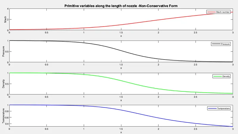
1`>>`Flow field vaiables along the length of Nozzle

Non-conservative form

Conservative form

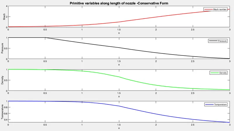
Observation: The above plots are almost same , when compared with the analytical solution from John D Anderson book.

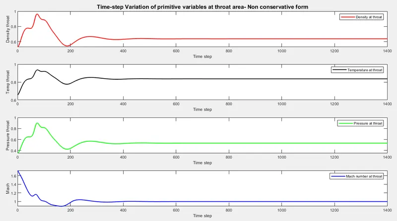
2`>>`Time wise variations of flow field variables at nozzle throat (Area=1)

Non-sonservative form

Conservative form

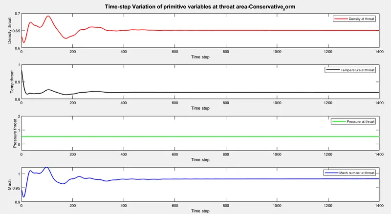
Observation: In this above plots of time step variation of primitive variables at throat area of non-conservative and conservative form , we observed that initially the plots are oscillating most and after almost 500 time steps it started to achieve the stable solution. By this you can note that non conservative form reaches steady state earlier than conservative form.

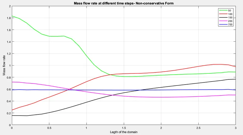
3`>>`Variations of mass flow rate distributions througuh the nozzle at different times

Non-conservative form

Conservative form

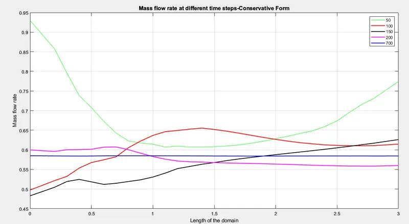
Observation: Above plots shows that Mass Flow Rate at different Time steps along the Nozzle oscillates initially, however the solution becomes stable after the 700th Timestep for both the forms Non-conservative and conservative.

4`>>`Mass flow variations obtained from the non-conservations and conservations form of governing equations

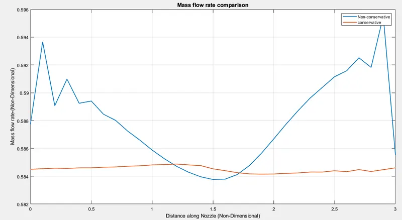
Observation: In this above plot we can see the steady state mass flow variations along the nozzle length obtained with the non-conservation and conservation governing equations. By seeing this plot, we can say that the conservation form gives a distribution that is much closer to being a constant. But, the non-conservation results have a sizeable variation, with some oscillations at both inlet and outlet boundaries. The latter also gives almost stable solution along the length. By this we can conclude that Conservative form attains stability in lesser number of iterations with earliest time.

Grid dependency test and comparing the results with Analytical solution

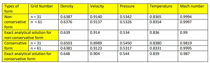
This is Grid dependency test, where, analysis begins with a coarse mesh and it is refined to finer mesh for each run until the results do not change significantly and depend of the grid size anymore. As the grid or mesh size approaches zero, the approximate solution is almost equal to the actual solution.

It is clear from the above table that the values are almost same along all the Primitive Variables for both the forms even when the Grid points(n) is changed from 31 to 61. The solution doesn't get affected by the increase of Grid points. So, we can cleary conclude that, the above problem is grid independence.

Also it can be seen from the comparison table, that non-conservative solutions give more accurate results than the conservative solution.

Conclusion :

• We have solved the 1D quasi subsonic-supersonic nozzle flow problem using MacCormack's technique numerically in both forms Non-conservation and Conservation.
• Plotting has been done of flow field variables (Density, Pressure, Temperature, Mach number) along the Nozzle length and also at different time steps. Also, we have looked at the distributiond of primitive variables with time steps at Nozzle throat location (Area = 1).
• We have done grid dependency test by changing the number of grid points from 31 to 61 and compared the results with Exact analytical solution.
• After the completion of entire solution, we can conclude that we cannot establish a clear superiority of one form over one form. Because, we can see that conservaive form gives a better mass flow distributions along the nozzle length. But, non-conservative forms have a sizeable variation, with some oscillations at both inlet and outlet boundaries. In another observation, we observed from comparison with the exact analytical solution that non-conservative form gives more accurate result compared to conservative form.
• Non-conservative form attains steady state faster than the conservative form.
• And, from the grid dependency test, we can come to this conclusion that, both the forms are grid independent.