Challenge

Week 7 - Simulation of a 1D Supersonic nozzle flow simulation using Macormack Method

JJaweria S25 Feb 2023

AIM:

To simulate the isentropic flow through a quasi 1D subsonic-supersonic nozzle, for both conservative and non-conservative forms of governing equations using the MacCormack's technique.

THEORY:

Convergent-Divergent Nozzle

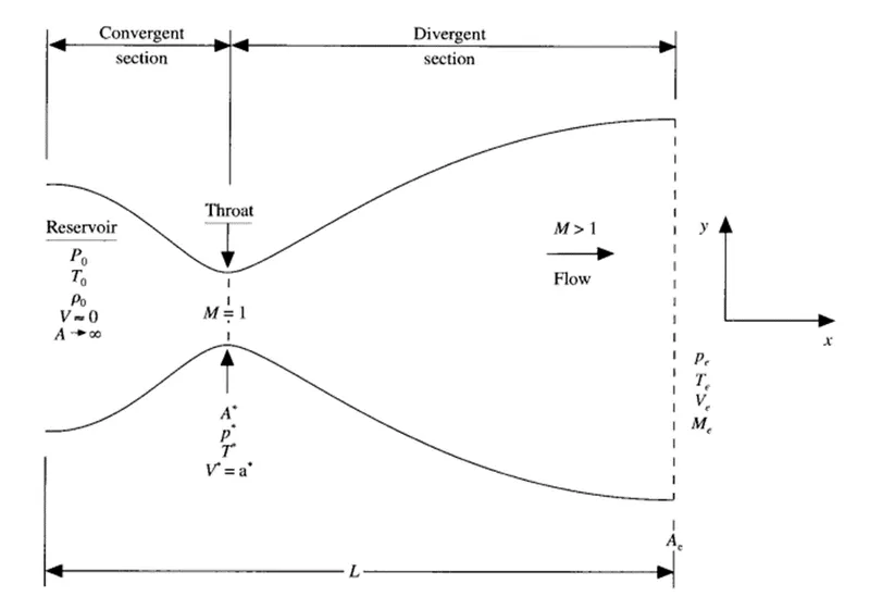
Consider isentropic flow through Subsonic-Supersonic nozzle, also known as Convergent-Divergent nozzle. At nozzle inlet flow comes from a reservoir with a very low velocity (i.e. V = 0 m/s) with initial parameters as pressure (Po) and temperature (To), flow entered through the nozzle travels through the convergent section, where flow is locally subsonic (M < 1).

In throat section with the gradual decrease in the cross-section area the area reaches to a critcial area, where the velocity reaches from subsonic to sonic (M = 1), At the throat the velocity of the fluid reaches to the speed of sound denoted by (a∗), area (A∗), pressure (P∗) and temperature (T∗).

The velocity of fluid increases with the increase in area in divergent section the velocity of the fluid goes Super-Sonic and parameters as pressure (Pe), temperature (Te), Velocity (Ve) and Area (Ae).

Convergent Section: M < 1 Subsonic flow

Throat Section: M = 1 Sonic flow

Divergent Section: M > 1 Supersonic flow

Governing Equation

The Governing Equation for the Quasi One-Dimensional, Steady, Inviscid, Isentropic Flow is as follows,

Continuity Equation: `ρ_(1 . ) V_(1 . ) A_(1 = ) ρ_(2 . ) V_(2 . ) A_(1 )`

Momentum Equation: `p_(1 . ) A_(1 )+ρ_(1 . ) V_1^2 .A_(1 )+ ∫_(A_2)^(A_1)▒〖p . dA 〗= p_(2 . ) A_(2 + ) ρ_(2 . ) V_2^2 .A_(2 )`

Energy Equation: `h_(1 )+ (V_1^2)/2= h_(2 )+ (V_2^2)/2`

We assume that flow is quasi one-dimensional flow i.e., at a given cross-sectional area A, all flow variables vary primarily along one direction, say x, the flow properties are uniform across this section. But in reality the flow field is two-dimensional (the flow varies in the two-dimensional x-y space).

Partial Differential Form of the Governing Equations

Consider a small control volume as shown in figure below for deriving partial differential equations for quasi 1-D Subsonic Supersonic nozzle flow.

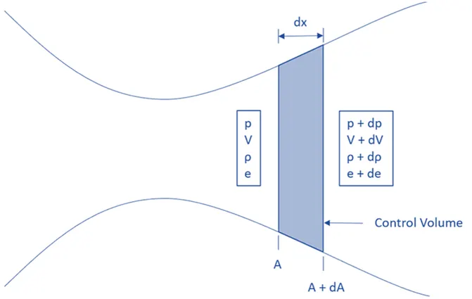
Governing Equations are represented in terms of PDE for both forms, to use Time Marching solution.

The continuity, momentum, and energy governing equations for this quasi-one-dimensional unsteady isentropic flow can be expressed respectively as

Non-Conservation Form - Control Volume is moving along the fluid.

Continuity Equation: `(∂(ρA))/∂t+ ρA ∂V/∂x+ρV ∂A/∂x+ VA ∂ρ/∂x=0`

Momentum Equation: `ρ ∂V/∂t+ρV ∂V/∂t = - R ( ρ ∂T/∂x+T ∂ρ/∂x )`

Energy Equation: `ρ C_(v ) ∂T/∂t+ ρ V C_(v ) ∂T/∂x = - ρRT ( ∂V/∂x+V (∂(ln⁡〖A)〗)/∂x )`

Conservative Form - Control Volume is stationary

Continuity Equation: `(∂(ρA))/∂t+ (∂(ρAV))/∂x=0`

Momentum Equation: `(∂(ρAV))/∂t+ (∂(ρAV^2))/∂x= -A ∂ρ/∂x`

Energy Equation: `(∂(ρ. A. (e + V^2/2)))/∂t + (∂(ρ. A. V.(e + V^2/2) + pAV))/∂x=0`

Non – Dimensional Form of Partial Differential Governing Equations

Converting equations to non-dimensional form, to reduce the number of variables that describe a system, thereby reducing the amount of experimental data required to make correlations of physical phenomena to scalable systems.

Non-Dimensional Variable for the governing equation with respect to the Flow-Field Variables are as follows,

`T^(' )= T/T_o , ρ^(' )= ρ/ρ_o , V^(' )= V/a_o , A^(' )= A/A^* , x^(' )= x/L , t^(' )= t/(L/a_o )`

Here,

T = Temperature of fluid

T_o= Temperature at the reservoir

ρ = Density of fluid

ρ_o= Density at the reservoir

V = Velocity of fluid

= Speed of sound at the reservoir

A = Cross sectional area of nozzle

= Cross sectional area at the throat

x = Location of nozzle

L = length of nozzle

t = time

Non-Conservation Form - Control Volume is moving along the fluid.

Continuity Equation: `(∂ρ^')/(∂t^' )= - ρ^' (∂V^')/(∂x^' )- ρ^' V^' (∂〖(ln⁡A〗^'))/(∂x^' )- V^' (∂ρ^')/(∂x^' )`

Momentum Equation: `(∂V^')/(∂t^' )= - V^' (∂V^')/(∂x^' )- 1/γ ((∂T^')/(∂x^' )+ T^'/ρ^' . (∂ρ^')/(∂x^' ))`

Energy Equation: `(∂T^')/(∂t^' )= - V^' (∂T^')/(∂x^' )-(γ-1).T^' ((∂V^')/(∂x^' )+ V^' . (∂(lnA^'))/(∂x^' ))`

Conservative Form - Control Volume is stationary

Continuity Equation: `(∂〖(ρ〗^' A^'))/(∂t^' )+ (∂〖(ρ〗^' A^' V^'))/(∂x^' )=0`

Momentum Equation: `(∂〖(ρ〗^' A^' V^'))/(∂t^' ) + (∂〖(ρ〗^' A^' V^('2 )+(1/γ) p^' A^'))/(∂x^' )= 1/γ .p^' (∂A^')/(∂x^' )`

Energy Equation: `(∂〖(ρ〗^' A^' (e^'/(γ-1) + γ/2 V^('2 ) )))/(∂t^' ) + (∂〖(ρ〗^' A^' V^' (e^'/(γ-1) + γ/2 V^('2 ) ) + p^' A^' V^'))/(∂x^' )=0`

Simplifying Conservative Form

Continuity Equation: `(∂U_1)/(∂t^' ) = - (∂F_1)/(∂x^' )`

Momentum Equation: `(∂U_2)/(∂t^' ) = - (∂F_2)/(∂x^' )+ J_2`

Energy Equation: `(∂U_3)/(∂t^' ) = - (∂F_3)/(∂x^' )`

Solution Vectors:

`U1 =ρ^' A^'`

`U2 =ρ^' A^' V^'`

`U3 = ρ^' A^' (e^'/(γ-1) + γ/2 V^('2 ) )`

Flux Vectors:

`F1 =ρ^' A^' V^'`

`F2 = ρ^' A^' V^'2+(1/γ) p^' A^'`

`F3 = ρ^' A^' V^' (e^'/(γ-1) + γ/2 V^('2 ) ) + p^' A^' V^'`

Source Term:

`J2 = 1/γ .p^' (∂A^')/(∂x^' )`

Here,

`ρ^'= U_1/A^'`

`V^'= U_2/U_1`

`T^'= e^'=(γ-1) (U_3/U_1 - γ/2 V^('2 ) )`

`p^'= ρ^' T^'`

Following steps are followed to simulate the flow through quasi one dimensional Subsonic Supersonic nozzle.

Mesh Generation:

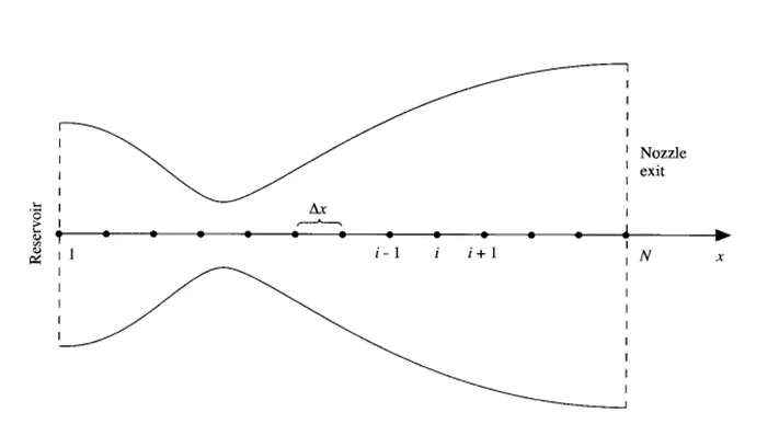
In the process, dividing a continuous geometry into discrete geometric cells, Each cell is separated by a node. These nodes form The Grid.

We assumed Quasi 1-D Nozzle Flow, So To implement a finite-difference solution, we divide the Nozzle length into a number of discrete grid points along the X – direction, This assumption of Quasi-1D and Inviscid reduces the complexity for the grid generation.

Discretization:

In this process, converting the above PDEs into algebraic equations, using MacCormack Technique for the Discretization.

MacCormack method is a second-order explicit finite difference technique, widely used discretization scheme for the numerical solution of hyperbolic partial differential equations.

MacCormack is predictor corrector method and is second order accurate in both space and time.

Solving:

Initial Condition

Initial conditions are guess values, to determine the profile of flow field variables like velocity, density, and temperature.

Predictor Step

Discretizing the governing equation using the forward difference method. We set the spatial derivatives as forward differences, and calculate the time derivative terms.

`(∂f/∂t)_p= (f(i+1)-f(i))/Δx`

Solution Update

From the time derivate, updating the values of primitive variables.

`fp = fintial + (∂f/∂t)_p . Δt`

Corrector Step

Discretizing the equations using the backward difference and from the predicted values of the flow variables from the predictor step.

`((∂f_p)/∂t)_c= (f(i)-f(i-1))/Δx`

Average derivatives

Computing the average of the time derivatives of governing equations solved by the predictor and corrector method.

`(∂f/∂t)_(avg )=0.5 ((∂f/∂t)_p+ ((∂f_p)/∂t)_c )`

Final Solution Update

Updating the primitive variable terms and obtaining the final corrected values, by the average time derivatives.

`fsol = fintial + (∂f/∂t)_avg . Δt`

Initial Conditions and Boundary Conditions

The nozzle shape, A = A(x) is specified and held fixed, independent of time.

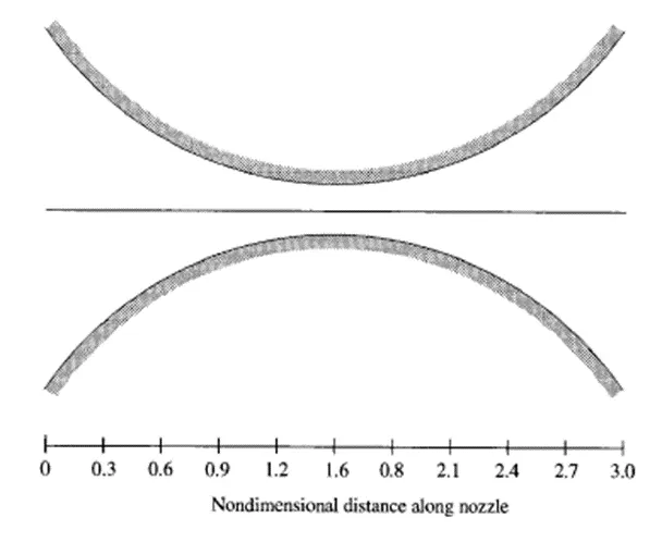
For this project the area is taken in the form of a parabolic curve which is denoted by `A = 1 + 2.2 (x – 1.5)2`

The throat of the nozzle is at x = 1.5, the convergent section occurs at x < 1.5 and the divergent section occurs at x > 1.5, parabolic curve can be seen in below figure.

We try to simulate the program for a time of 1400 time steps and the length of the nozzle is taken as 3 units which is divided into 31 nodes. The time step provided is such that it satisfies the CFL criteria.

Initial condition and Boundary condition, Non-Conservation Form

Initial condition

ρ = 1 – 0.3146 * x

T = 1 – 0.2314 * x

`v = (0.1 + 1.09 * x) * √T`

Boundary condition

Inlet:

v(1) = 2 * v(2) - v(3)

Outlet:

`ρ(n) = 2 * ρ(n-1) - ρ(n-2)`

`T(n) = 2 * T(n-1) - T(n-2)`

`v(n) = 2 * v(n-1) - v(n-2)`

Initial condition and Boundary condition, Conservative Form

Initial condition

For 0 ≤ x ≤ 0.5 `〖 ρ〗^' = 1.0 ; T^'=1.0`

For 0.5 ≤ x ≤ 1.5 `〖 ρ〗^'=1.0-0.366(x^'-0.5); 〖 T〗^'=1.0-0.167(x^'-0.5)`

For 1.5 ≤ x ≤ 3.5 `〖 ρ〗^'=0.634-0.3879(x^'-1.5); 〖 T〗^'=0.833-0.3507(x^'-1.5)`

Boundary condition

Inlet:

`U1(1)= ρ^' (1)*a^' (1)`

`U2(1)= 2*U2(2)-U2(3)`

`U3(1)= U1(1)* ((T(1))/((γ-1))+ γ/2*v(〖1)〗^2 )`

Outlet:

`U1(n)= 2*U1(n-1)-U2(n-2)`

`U2(n)= 2*U2(n-1)-U2(n-2)`

`U3(n)= 2*U3(n-1)-U3(n-2)`

MATLAB CODE

Main Program

% 1D QUASI SUBSONIC SUPERSONIC NOZZLE FLOW 

clear all
close all
clc

% Inputs

n = 31; % Number of grid points                 
gamma = 1.4;
x = linspace(0,3,n);
dx = x(2) - x(1);
nt = 1400; % Definning time steps
C = 0.5; % Courant Number           


% Function call for Non Conservative form
tic;
[Mass_flow_rate_nc, Pressure_nc, Mach_number_nc, rho_nc, v_nc, T_nc, rho_throat_nc, v_throat_nc, T_throat_nc, Mass_flow_rate_throat_nc, Pressure_throat_nc, Mach_number_throat_nc] = non_conservative(x, dx, n, gamma, nt, C);
Time_elapsed_nc = toc;
fprintf('Time Elasped for Non Conservative form: %0.4f', Time_elapsed_nc);
hold on

% Plotting

figure(1)
% Timestep variation of properties at throat area (Non-Conservative form)

% Density
subplot(4,1,1)
plot(linspace(1,nt,nt),rho_throat_nc,'color','r')
ylabel('Density')
legend({'Density at throat'});
axis([0 1400 0 1.3]);
grid minor;
title('Timestep variation at throat area - NON CONSERVATIVE FORM')

% Temperature
subplot(4,1,2)
plot(linspace(1,nt,nt),T_throat_nc,'color','g')
ylabel('Temperature')
legend({'Temperature at throat'});
axis([0 1400 0.6 1]);
grid minor;

% Pressure
subplot(4,1,3)
plot(linspace(1,nt,nt),Pressure_throat_nc,'color','b')
ylabel('Pressure')
legend({'Pressure at throat'});
axis([0 1400 0.4 1.1]);
grid minor

% Mach Number
subplot(4,1,4)
plot(linspace(1,nt,nt),Mach_number_throat_nc,'color','k')
xlabel('Timesteps')
ylabel('Mach Number')
legend({'Mach Number at throat'});
axis([0 1400 0.6 1.4]);
grid minor;


figure(2);
% Steady state simulation for primitve values (Non-Conservative form)

% Density
subplot(4,1,1);
plot(x,rho_nc,'color','r')
ylabel('Density')
legend({'Density'});
axis([0 3 0 1])
grid minor;
title('Variation of Flow Rate Distribution - NON CONSERVATIVE')

% Temperature
subplot(4,1,2);
plot(x,T_nc,'color','g')
ylabel('Temperature')
legend({'Temperature'});
axis([0 3 0 1])
grid minor;

% Pressure
subplot(4,1,3);
plot(x,Pressure_nc,'color','b')
ylabel('Pressure')
legend({'Pressure'});
axis([0 3 0 1])
grid minor;

% Mach number
subplot(4,1,4);
plot(x,Mach_number_nc,'color','k')
xlabel('Nozzle Length')
ylabel('Mach number')
legend({'Mach number'});
axis([0 3 0 4])
grid minor;

% Function call for Conservative Form
tic;
[Mass_flow_rate_c, Pressure_c, Mach_number_c,  rho_c, v_c, T_c, rho_throat_c, v_throat_c, T_throat_c, Mass_flow_rate_throat_c, Pressure_throat_c, Mach_number_throat_c] = conservative(x, dx, n, gamma, nt, C);
Time_elasped_c = toc;
fprintf('Time Elasped for Conservative form: %0.4f', Time_elasped_c);

% Plotting

figure(3)
% Timestep variation of properties at throat area (Conservative form)

% Density
subplot(4,1,1)
plot(rho_throat_c,'color','r')
ylabel('Density')
legend({'Density at throat'});
axis([0 1400 0 1]);
grid minor;
title('Timestep variation at throat area - CONSERVATIVE FORM')

% Temperature
subplot(4,1,2)
plot(T_throat_c,'color','g')
ylabel('Temperature')
legend({'Temperature at throat'});
axis([0 1400 0.6 1]);
grid minor;

% Pressure
subplot(4,1,3)
plot(Pressure_throat_c,'color','b')
ylabel('Pressure')
legend({'Pressure at throat'});
axis([0 1400 0.2 0.8]);
grid minor

% Mach Number
subplot(4,1,4)
plot(Mach_number_throat_c,'color','k')
xlabel('Timesteps')
ylabel('Mach Number')
legend({'Mach Number at throat'});
axis([0 1400 0.6 1.4]);
grid minor;


figure(4);
% Steady state simulation for primitve values (Conservative form)

% Density 
subplot(4,1,1);
plot(x,rho_c,'color','r')
ylabel('Density')
legend({'Density'});
axis([0 3 0 1])
grid minor;
title('Variation of Flow Rate Distribution - CONSERVATIVE FORM')

% Temperature 
subplot(4,1,2);
plot(x,T_c,'color','g')
ylabel('Temperature')
legend({'Temperature'});
axis([0 3 0 1])
grid minor;

% Pressure
subplot(4,1,3);
plot(x,Pressure_c,'color','b')
ylabel('Pressure')
legend({'Pressure'});
axis([0 3 0 1])
grid minor;

% Mach number
subplot(4,1,4);
plot(x,Mach_number_c,'color','k')
xlabel('Nozzle Length')
ylabel('Mach number')
legend({'Mach number'});
axis([0 3 0 4])
grid minor;


figure(5)
% Mass Flow Rate Comparison Plot

hold on
plot(x,Mass_flow_rate_nc,'r','linewidth',2)
hold on;
plot(x,Mass_flow_rate_c,'k','linewidth',2)
hold on;
grid on
legend('Non Conservative','Conservative');
xlabel('Length of the Domain')
ylabel('Mass Flow Rate')
title('Comparison of Mass Flow Rate of both forms')

Function Program for Non Conservative Form

% Function code for Non Conservative form

function [Mass_flow_rate_nc, Pressure_nc, Mach_number_nc, rho_nc, v_nc, T_nc, rho_throat_nc, v_throat_nc, T_throat_nc, Mass_flow_rate_throat_nc, Pressure_throat_nc, Mach_number_throat_nc] = non_conservative(x, dx, n, gamma, nt, C)

% Initial conditions

rho_nc = 1 - 0.3146*x;
T_nc = 1 - 0.2314*x;
v_nc = (0.1 + 1.09*x).*T_nc.^0.5;
a = 1 + 2.2*(x - 1.5).^2; % Area
throat = find(a==1); % Throat


% Outer Time Loop
for k = 1:nt
    
    % Time-step control
    dt = min(C.*dx./(sqrt(T_nc) + v_nc));
    
    % Saving a copy of Old Values
    rho_old = rho_nc;
    T_old = T_nc;
    v_old = v_nc;
    

   % Step 1 - Predictor method (forward difference for space terms)
    for j = 2:n-1
        
        % Simplifying the Equation's spatial terms
        dv_dx = (v_nc(j + 1) - v_nc(j))/dx;
        drho_dx = (rho_nc(j + 1) - rho_nc(j))/dx;
        dT_dx = (T_nc(j + 1) - T_nc(j))/dx;
        dlog_a_dx = (log(a(j + 1)) - log(a(j)))/dx;
        
        % Solving for continuity Equation
        drho_dt_p(j) = -rho_nc(j)*dv_dx - rho_nc(j)*v_nc(j)*dlog_a_dx - v_nc(j)*drho_dx;
        
        % Solving for momentum Equation
        dv_dt_p(j) = -v_nc(j)*dv_dx - (1/gamma)*(dT_dx + (T_nc(j)*drho_dx/rho_nc(j)));
        
        % Solving for energy Equation
        dT_dt_p(j) = -v_nc(j)*dT_dx - (gamma - 1)*T_nc(j)*(dv_dx + v_nc(j)*dlog_a_dx);
        
        
        % Step 2 - Solution update
        rho_nc(j) = rho_nc(j) + drho_dt_p(j)*dt;
        v_nc(j) = v_nc(j) + dv_dt_p(j)*dt;
        T_nc(j) = T_nc(j) + dT_dt_p(j)*dt;
        
    end
    
    
    % Step 3 - Corrector method (backward difference for space terms)
    for j = 2:n-1
        
        % Simplifying the Equation's spatial terms
        dv_dx = (v_nc(j) - v_nc(j - 1))/dx;
        drho_dx = (rho_nc(j) - rho_nc(j - 1))/dx;
        dT_dx = (T_nc(j) - T_nc(j - 1))/dx;
        dlog_a_dx = (log(a(j)) - log(a(j - 1)))/dx;
        
        % Continuity Equation
        drho_dt_c(j) = - rho_nc(j)*dv_dx - rho_nc(j)*v_nc(j)*dlog_a_dx - v_nc(j)*drho_dx;
        
        % Momentum Equation
        dv_dt_c(j) = - v_nc(j)*dv_dx - (1/gamma)*(dT_dx + (T_nc(j)*drho_dx/rho_nc(j)));
        
        %Energy Equation
        dT_dt_c(j) = - v_nc(j)*dT_dx - (gamma - 1)*T_nc(j)*(dv_dx + v_nc(j)*dlog_a_dx);
       
    end
    
    % Step 4 - Averaging predictor and corrector method
    drho_dt = 0.5.*(drho_dt_p + drho_dt_c);
    dv_dt = 0.5.*(dv_dt_p + dv_dt_c);
    dT_dt = 0.5.*(dT_dt_p + dT_dt_c);
    
    % Step 5 - Final solution update 
    for i = 2:n-1
        rho_nc(i) = rho_old(i) + drho_dt(i)*dt;
        v_nc(i) = v_old(i) + dv_dt(i)*dt;
        T_nc(i) = T_old(i) + dT_dt(i)*dt;
        
    end
    
    % Boundary Conditions
    % At Inlet
    rho_nc(1) = 1;
    v_nc(1) = 2*v_nc(2) - v_nc(3);
    T_nc(1) = 1;
    
    % At Outlet
    rho_nc(n) = 2*rho_nc(n-1) - rho_nc(n - 2);
    v_nc(n) = 2*v_nc(n - 1) - v_nc(n - 2);
    T_nc(n) = 2*T_nc(n - 1) - T_nc(n - 2);
    
    
    % Defining flow properties
    Mass_flow_rate_nc = rho_nc.*a.*v_nc;
    Pressure_nc = rho_nc.*T_nc;
    Mach_number_nc = (v_nc./sqrt(T_nc));
    
    % Calculating Variables at throat section
    rho_throat_nc(k) = rho_nc(throat);
    T_throat_nc(k) = T_nc(throat);
    v_throat_nc(k) = v_nc(throat);
    Mass_flow_rate_throat_nc(k) = Mass_flow_rate_nc(throat);
    Pressure_throat_nc(k) = Pressure_nc(throat);
    Mach_number_throat_nc(k) = Mach_number_nc(throat);
    
    
    % Plotting
    % Comparison of non-dimensional Mass flow rates at different time steps
    figure(6);
    if k == 1
       plot(x, Mass_flow_rate_nc, 'm', 'linewidth', 2);
       hold on
    elseif k == 50
       plot(x, Mass_flow_rate_nc, 'c', 'linewidth', 2);
       hold on
    elseif k == 100
       plot(x, Mass_flow_rate_nc, 'b', 'linewidth', 2);
       hold on
    elseif k == 200
       plot(x, Mass_flow_rate_nc, 'g', 'linewidth', 2);
       hold on
    elseif k == 400
       plot(x, Mass_flow_rate_nc, 'r', 'linewidth', 2);
       hold on
    elseif k == 800
       plot(x, Mass_flow_rate_nc, 'y', 'linewidth', 2);
       hold on
    elseif k == 1000
       plot(x, Mass_flow_rate_nc, 'k', 'linewidth', 2);
       hold on
    end
    
    title('Mass flow rates at different Timesteps - NON CONSERVATIVE FORM')
    xlabel('Distance')
    ylabel('Mass flow rate')
    legend('1st Timestep','5oth Timestep','100th Timestep','200th Timestep','400th Timestep','800th Timestep','1000th Timestep');
    grid on
    
end

end

Function Program for Conservative Form

% Function code for Conservative form

function [Mass_flow_rate_c, Pressure_c, Mach_number_c,  rho_c, v_c, T_c, rho_throat_c, v_throat_c, T_throat_c, Mass_flow_rate_throat_c, Pressure_throat_c, Mach_number_throat_c] = conservative(x, dx, n, gamma, nt, C)

% Initial Conditions 
for i = 1:n
    
    if (x(i) >= 0 && x(i) <= 0.5)
        rho_c(i) = 1;
        T_c(i) = 1;
    elseif (x(i) >= 0.5 && x(i) <= 1.5)
        rho_c(i) = 1 - 0.366*(x(i) - 0.5);
        T_c(i) = 1 - 0.167*(x(i) - 0.5);
    elseif (x(i) >= 1.5 && x(i) <= 3)
        rho_c(i) = 0.634 - 0.3879*(x(i) - 1.5);
        T_c(i) = 0.833 - 0.3507*(x(i) - 1.5);
    end
    
end

a = 1 + 2.2*(x - 1.5).^2; % Area
throat = find(a==1); % Throat

% Initial Velocity and Pressure
v_c = 0.59./(rho_c.*a);
Pressure_c = rho_c.*T_c;

% Solution Vectors(U)
U1 = rho_c.*a;
U2 = rho_c.*a.*v_c;
U3 = rho_c.*a.*(T_c./(gamma - 1)) + ((gamma/2).*v_c.^2);


% Outer Time Loop
for k =1:nt
    
    % Time-step control
    dt = min(C.*dx./(sqrt(T_c) + v_c));
    
    % Saving a copy of Old Values
    U1_old = U1;
    U2_old = U2;
    U3_old = U3;

    % Calculating the Flux vector(F)
    F1 = U2;
    F2 = ((U2.^2)./U1) + ((gamma - 1)/gamma)*(U3 - (gamma/2)*((U2.^2)./U1));
    F3 = ((gamma*U2.*U3)./U1) - (gamma*(gamma - 1)*((U2.^3)./(2*U1.^2)));
    
    
    % Step 1 - Predictor method (forward difference for space terms)
    for j = 2:n-1
    
        %Calculating the Source term(J)
        J2(j) = (1/gamma)*rho_c(j)*T_c(j)*((a(j + 1) - a(j))/dx);
        
        
        % Solving for continuity Equation
        dU1_dt_p(j) = -((F1(j + 1) - F1(j))/dx);
        
        % Solving for momentum Equation
        dU2_dt_p(j) = -((F2(j + 1) - F2(j))/dx) + J2(j);
        
        % Solving for energy Equation
        dU3_dt_p(j) = -((F3(j + 1) - F3(j))/dx);
        
        
        % Step 2 - Solution update
        U1(j) = U1(j) + dU1_dt_p(j)*dt;
        U2(j) = U2(j) + dU2_dt_p(j)*dt;
        U3(j) = U3(j) + dU3_dt_p(j)*dt;
        
    end
    
    % Updating Flux vectors
    F1 = U2;
    F2 = ((U2.^2)./U1) + ((gamma - 1)/gamma)*(U3 - ((gamma*0.5*(U2.^2))./(U1)));
    F3 = ((gamma*U2.*U3)./U1) - ((gamma*0.5*(gamma - 1)*(U2.^3))./(U1.^2));

    
   % Step 3 - Corrector method (backward difference for space terms)
    for j = 2:n-1
        
        % Updating the Source term(J)
        J2(j) = (1/gamma)*rho_c(j)*T_c(j)*((a(j) - a(j - 1))/dx);

        % Solving for continuity Equation
        dU1_dt_c(j) = -((F1(j) - F1(j - 1))/dx);
        
        % Solving for momentum Equation
        dU2_dt_c(j) = -((F2(j) - F2(j - 1))/dx) + J2(j);
        
        % Solving for energy Equation
        dU3_dt_c(j) = -((F3(j) - F3(j - 1))/dx);

    end

    % Step 4 - Averaging predictor and corrector method
    dU1_dt = 0.5*(dU1_dt_p + dU1_dt_c);
    dU2_dt = 0.5*(dU2_dt_p + dU2_dt_c);
    dU3_dt = 0.5*(dU3_dt_p + dU3_dt_c);

    % Step 5 - Final solution update 
    for i = 2:n-1
        U1(i) = U1_old(i) + dU1_dt(i)*dt;
        U2(i) = U2_old(i) + dU2_dt(i)*dt;
        U3(i) = U3_old(i) + dU3_dt(i)*dt;
        
    end
    
    % Boundary Conditions
    % At Inlet
    U1(1) = rho_c(1)*a(1);
    U2(1) = 2*U2(2) - U2(3);
    
    v_c(1) = U2(1)./U1(1);
    U3(1) = U1(1)*((T_c(1)/(gamma - 1)) + ((gamma/2)*(v_c(1)).^2));
    
    % At Outlet
    U1(n) = 2*U1(n - 1) - U1(n - 2);
    U2(n) = 2*U2(n - 1) - U2(n - 2);
    U3(n) = 2*U3(n - 1) - U3(n - 2);
    
    % Final Primitive value update
    rho_c = U1./a;
    v_c = U2./U1;
    T_c = (gamma - 1)*((U3./U1 - (gamma/2)*(v_c).^2));
    
    % Defining flow properties
    Mass_flow_rate_c = rho_c.*a.*v_c;
    Pressure_c = rho_c.*T_c;
    Mach_number_c = (v_c./sqrt(T_c));
    
    % Calculating Variables at throat section
    rho_throat_c(k) = rho_c(throat);
    T_throat_c(k) = T_c(throat);
    v_throat_c(k) = v_c(throat);
    Mass_flow_rate_throat_c(k) = Mass_flow_rate_c(throat);
    Pressure_throat_c(k) = Pressure_c(throat);
    Mach_number_throat_c(k) = Mach_number_c(throat);

    % Plotting
    % Comparison of non-dimensional Mass flow rates at different time steps
    figure(7)
    if k == 1
       plot(x, Mass_flow_rate_c, 'm', 'linewidth', 2);
       hold on
    elseif k == 50
       plot(x, Mass_flow_rate_c, 'c', 'linewidth', 2);
       hold on
    elseif k == 100
       plot(x, Mass_flow_rate_c, 'b', 'linewidth', 1.25);
       hold on
    elseif k == 200
       plot(x, Mass_flow_rate_c, 'g', 'linewidth', 1.25);
       hold on
    elseif k == 400
       plot(x, Mass_flow_rate_c, 'r', 'linewidth', 1.25);
       hold on
    elseif k == 800
       plot(x, Mass_flow_rate_c, 'y', 'linewidth', 1.25);
       hold on
    elseif k == 1000
       plot(x, Mass_flow_rate_c, 'k', 'linewidth', 2);
       hold on
    end
  
    title('Mass flow rates at different Timesteps - CONSERVATIVE FORM')
    xlabel('Distance')
    ylabel('Mass flow rate')
    legend('1st Timestep','5oth Timestep','100th Timestep','200th Timestep','400th Timestep','800th Timestep','1000th Timestep');
    axis([0 3 0.4 1])
    grid on
    
end

end

OUTPUT

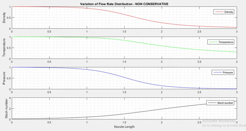
1. Variation of flow rate distribution throughout the nozzle length for both Non Conservative and Conservative form

Non Conservative form

Conservative form

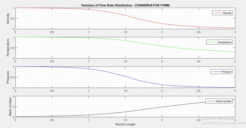
In the above figures we can see how the variables change over the non dimensionalized distance. We can observe that at the throat section i.e., at x’ = 1.5 the mach number seems to increase indicating the flow is changing from subsonic to supersonic over the nozzle, The pressure is compensated for an increase in velocity. The variation in flow distribution throughout the length of the nozzle is the same for both forms.

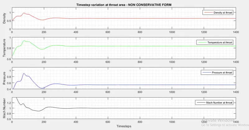
2. Variations of flow properties at Throat area at different timesteps for both Non Conservative and Conservative form

Non Conservative form

Conservative form

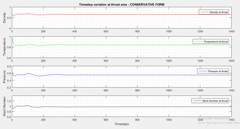
From the above figures we can say that both conservative and non-conservative forms have deviations in the beginning of the time marching, but the conservative form had relatively less deviations compared to non-conservative flow. Over the time both have converged into a stable solution.

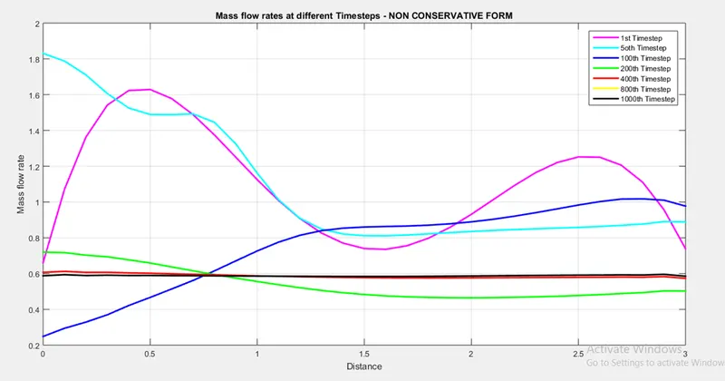
3. Mass flow rate at different timesteps for both Non Conservative and Conservative form

Non Conservative form

Conservative form

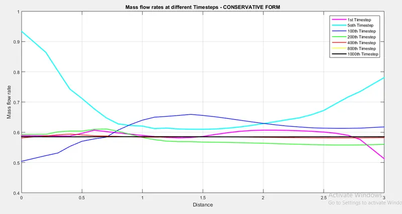
From the above figures we can observe that the mass flowrate tends to stabilise from 400th timestep and at 1000^th timestep it is completely stable for both the forms, also we can observe that the Non conservative mass flow rate has more deviation than the conservative timestep this might be due to the reason that the control volume is moving in conservative.

4. Comparison of mass flow rate for both Non Conservative and Conservative forms

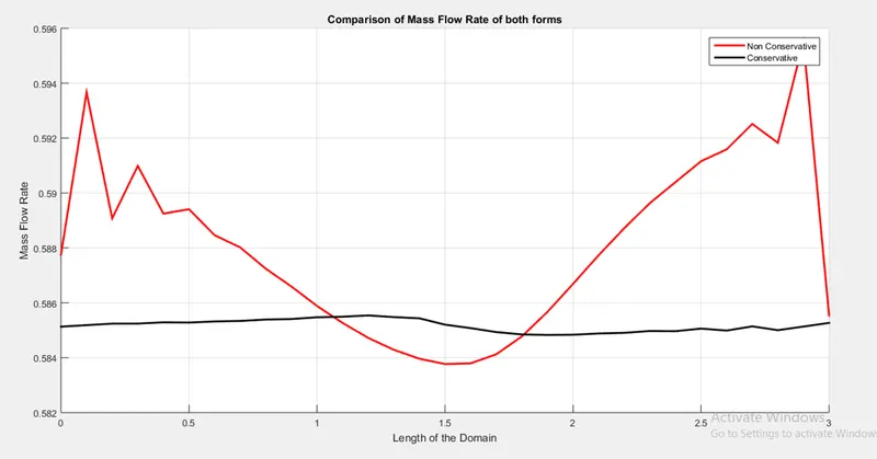
From the above graph it is observed that the mass flow rate for both the process are very much near to analytical solution. The Non Conservative mass flow rate is deviating more than the conservative mass flow rate hence in a study about mass flow rate the conservative form is much more reliable than the non-conservative form.

GRID INDEPENDENCE TEST

Non Conservative form

Number of grid points	Density	Temperature	Pressure	Mach Number
31	0.6387	0.8365	0.5342	0.9994
61	0.6376	0.8354	0.5326	0.9997

Conservative form

Number of grid points	Density	Temperature	Pressure	Mach Number
31	0.6516	0.8406	0.5478	0.9795
61	0.6383	0.8351	0.5331	0.9992

The above values are precise to two digits after the decimal we can say that the solution is grid independent. If all the four digits after the decimal are not precise then the solution becomes grid dependent.

CONCLUSION

From the above data we can conclude that the Conservative form is much more accurate and reliable than non-conservative form. In order for us to achieve more accurate results with the non-conservative the timesteps must be increased.

Week 7 - Simulation of a 1D Supersonic nozzle flow simulation using Macormack Method

Ship work like this
in your own course.

Talk to a career counsellor

Ship work like thisin your own course.

Talk to a career counsellor

Ship work like this
in your own course.