Week 3.5 - Deriving 4th order approximation of a 2nd order derivative using Taylor Table method

Aim: To derive and write a MATLAB program for the second order derivative with fourth order approximations using central difference, skewed right sided difference and skewed left sided difference method.

Objective:

1. To derive the second order derivative, function given f(x) = exp(x)*cos(x). Proving that the skewed schemes are fourth order accurate.
2. To write a program in MATLAB to evaluate the second order derivative, function f(x) = exp(x)*cos(x). Compare it with approximations derived.
3. To plot a figure which compares absolute error between the schemes

Central Difference Method:

Function Given: f(x) = exp(x)*cos(x)

Second order derivation of above function: f’’(x) = -2*exp(x)*sin(x)

Order of accuracy for central scheme, provided: P = N – Q + 1

Where: P is Order of accuracy

N is Number of nodes in the stencil

Q is order of derivative

Therefore, number of nodes for second order of derivative with fourth order approximation for central scheme is: 4 = N – 2 + 1

N = 5

Taylor’s series expansion for central difference scheme

`(δ^2 f)/(δx^2 ) = af(i-2)+bf(i-1)+cf(i)+df(i+1)+ef(i+2)`

`af(i-2)=a[f(i) - 2Δx/1!*f’(i) + ((2Δ〖x)〗^2)/2!*f^'' (i)- ((2Δ〖x)〗^3)/3!*f^''' (i)+ ((2Δ〖x)〗^4)/4!*f^'''' (i)- ((2Δ〖x)〗^5)/5!*f^''''' (i)]`

`bf(i-1)=b[f(i) - Δx/1!*f’(i) + ((Δ〖x)〗^2)/2!*f^'' (i)- ((Δ〖x)〗^3)/3!*f^''' (i)+ ((Δ〖x)〗^4)/4!*f^'''' (i)- ((Δ〖x)〗^5)/5!*f^''''' (i)]`

`cf(i)=cf(i)`

`df(i+1)=d[f(i) + Δx/1!*f’(i) + ((Δ〖x)〗^2)/2!*f^'' (i)+ ((Δ〖x)〗^3)/3!*f^''' (i)+ ((Δ〖x)〗^4)/4!*f^'''' (i)+ ((Δ〖x)〗^5)/5!*f^''''' (i)]`

`ef(i+2)=e[f(i) +2Δx/1!*f’(i) + ((2Δ〖x)〗^2)/2!*f^'' (i)+ ((2Δ〖x)〗^3)/3!*f^''' (i)+ ((2Δ〖x)〗^4)/4!*f^'''' (i)+ ((2Δ〖x)〗^5)/5!*f^''''' (i)]`

As, we are solving for second derivative function, the sum of coefficients of f’’(i) equal to 1 and rest are zero.

From above equations finding coefficients a, b, c, d and e for central scheme

Above expansions can be formulated in tabular column called Taylors table for central scheme:

	f(i)	f’(i)	f’’(i)	f’’’(i)	f’’’’(i)	f’’’’’(i)	f’’’’’’(i)
a*f(i-2)	a	-2a	4a/2	-8a/6	2a/3	-4a/15	4a/45
b*f(i-1)	b	-b	b/2	-b/6	b/24	-b/120	b/720
c*f(i)	c	0	0	0	0	0	0
d*f(i+1)	d	d	d/2	d/6	d/24	d/120	d/720
e*f(i+2)	e	2e	4e/2	8e/6	2e/3	4e/15	4e/45
(Sum of above terms)	0	0	1	0	0	?	?

We require only 5 equations to find value of 5 coefficients (a, b, c, d and e), so the last two columns can be ignored.

Considering coefficients of 5 columns:

`a + b + c + d + e = 0`

`-2a – b + d + 2e = 0`

`4a/2+ b/2+ d/2 + 4e/2 = 1`

`-8a/6- b/6+ d/6 + 8e/6 = 0`

`2a/3+ b/24+ d/24 + 2e/3 = 0`

Writing above equations in matrix form: A.X = B

`⌊■(1&1&1&1&1@-2&-1&0&1&2@4/2&1/2&0&1/2&4/2@-8/6&-1/6&0&1/6&8/6@2/3&1/24&0&1/24&2/3)⌋`*`[■(a@b@c@d@e)]` = `[■(0@0@1@0@0)]`

Solving matrix by matrix inversion method to get value for coefficients a, b, c, d and e i.e., X = (inv)A*B

a = -0.83333

b = 1.33333

c = -2.50000

d = 1.33333

e = -0.83333

Substituting coefficient value in taylor’s series expansion

`(δ^2 f)/(δx^2 ) = af(i-2)+bf(i-1)+cf(i)+df(i+1)+ef(i+2)`

`(δ^2 f)/(δx^2 ) = (a + b + c + d + e)*f(i) + (-2a – b + d + 2e)*f’(i) + (4a/2 + b/2 + d/2 + 4e/2)*f’’(i) + (-8a/6 – b/6 + d/6 + 8e/6)*f’’’(i) + (2a/3 + b/24 + d/24 + 2e/3)*f’’’’(i) + (-4a/15 – b/120 + d/120 + 4e/15)*f’’’’’(i) + (4a/45 + b/720 + d/720 + 4e/45)*f’’’’’’(i)`

Considering a = e, b = d

`(δ^2 f)/(δx^2 ) = (a + b + c + b + e)*f(i) + (2a – b + b + 2a)*f’(i) + (4a/2 + b/2 + b/2 + 4a/2)*f’’(i) + (-8a/6 – b/6 + b/6 + 8a/6)*f’’’(i) + (2a/3 + b/24 + b/24 + 2a/3)*f’’’’(i) + (-4a/15 – b/120 + b/120 + 4a/15)*f’’’’’(i) + (4a/45 + b/720 + b/720 + 4a/45)*f’’’’’’(i)`

`(δ^2 f)/(δx^2 ) = 0 + 0 + 1*f’’(i)*dx2 + 0 + 0 + 0 + (8a/45 + b/360)*f’’’’’’(i)*dx6`

Dividing entire equation by dx² both sides

`(δ^2 f)/(δx^2 ) = f’’(i) + 0* dx4`

Hence, the above equation represents the fourth order central difference approximation for and the term 0*dx4 represents truncation error of fourth order.

Skewed Right-Sided Difference Method:

Function Given: f(x) = exp(x)*cos(x)

Second order derivation of above function: f’’(x) = -2*exp(x)*sin(x)

Order of accuracy for skewed right sided scheme, provided: P = N – Q

Where: P is Order of accuracy

N is Number of nodes in the stencil

Q is order of derivative

Therefore, number of nodes for second order of derivative with fourth order approximation for skewed right sided scheme is: 4 = N – 2

N = 6

Taylor’s series expansion for skewed right-Sided difference scheme

`(δ^2 f)/(δx^2 ) = a*f(i)+b*f(i+1)+c*f(i+2)+d*f(i+3)+e*f(i+4)+f*f(i+5)

`af(i)=af(i)`

`bf(i+1)=b[f(i) + Δx/1!*f’(i) + ((Δ〖x)〗^2)/2!*f^'' (i)+ ((Δ〖x)〗^3)/3!*f^''' (i)+ ((Δ〖x)〗^4)/4!*f^'''' (i)+ ((Δ〖x)〗^5)/5!*f^''''' (i)]`

`cf(i+2)=c[f(i)+ 2Δx/1!*f’(i) + ((2Δ〖x)〗^2)/2!*f^'' (i)+ ((2Δ〖x)〗^3)/3!*f^''' (i)+ ((2Δ〖x)〗^4)/4!*f^'''' (i)+ ((2Δ〖x)〗^5)/5!*f^''''' (i)]`

`df(i+3)=d[f(i) + 3Δx/1!*f’(i) + ((3Δ〖x)〗^2)/2!*f^'' (i)+ ((3Δ〖x)〗^3)/3!*f^''' (i)+ ((3Δ〖x)〗^4)/4!*f^'''' (i)+ ((3Δ〖x)〗^5)/5!*f^''''' (i)]

`ef(i+4)=e[f(i) +4Δx/1!*f’(i) + ((4Δ〖x)〗^2)/2!*f^'' (i)+ ((4Δ〖x)〗^3)/3!*f^''' (i)+ ((4Δ〖x)〗^4)/4!*f^'''' (i)+ ((4Δ〖x)〗^5)/5!*f^''''' (i)]`

`ff(i+5)=f[f(i) +5Δx/1!*f’(i) + ((5Δ〖x)〗^2)/2!*f^'' (i)+ ((5Δ〖x)〗^3)/3!*f^''' (i)+ ((5Δ〖x)〗^4)/4!*f^'''' (i)+ ((5Δ〖x)〗^5)/5!*f^''''' (i)]`

As, we are solving for second derivative function, the sum of coefficients of f’’(i) equal to 1 and rest are zero.

From above equations finding coefficients a, b, c, d, e and f for skewed right sided scheme

Above expansions can be formulated in tabular column called Taylors table for skewed right sided scheme:

	f(i)	f’(i)	f’’(i)	f’’’(i)	f’’’’(i)	f’’’’’(i)	f’’’’’’(i)
a*f(i)	a	0	0	0	0	0	0
b*f(i+1)	b	b	b/2	b/6	b/24	b/120	b/720
c*f(i+2)	c	2c	4c/2	8c/6	2c/3	4c/15	4c/45
d*f(i+3)	d	3d	9d/2	27d/6	81d/24	81d/40	81d/80
e*f(i+4)	e	4e	16e/2	64e/6	256e/24	128e/15	256e/45
f*f(i+5)	f	5f	25f/2	125f/6	625f/24	3125f/120	3125f/144
(Sum of above terms)	0	0	1	0	0	?	?

We require only 6 equations to find value of 6 coefficients (a, b, c, d, e and f), so the last one column can be ignored.

Considering coefficients of 6 columns:

`a + b + c + d + e + f = 0`

`b + 2c + 3d + 4e + 5f = 0`

`b/2+ 4c/2+ 9d/2 + 16e/2 +25f/2 = 1`

`b/6+ 8c/6+ 27d/6 + 64e/6+125f/6 = 0`

`b/24+ 2c/3+ 81d/24 + 256e/24+625f/24 = 0`

`b/120+ 4c/15+ 81d/40 + 128e/15+3125f/120 = 0`

Writing above equations in matrix form: A.X = B

`⌊■(1&1&1&1&1&1@0&1&2&3&4&5@0&1/2&4/2&9/2&16/2&25/2@0&1/6&8/6&27/6&64/6&125/6@0&1/24&2/3&81/24&256/24&625/24@0&1/120&4/15&81/40&128/15&3125/120)⌋`*`[■(a@b@c@d@e@f)]` = `[■(0@0@1@0@0@0)]`

Solving matrix by matrix inversion method to get value for coefficients a, b, c, d, e and f i.e., X = (inv)A*B

a = 3.7500

b = -12.833

c = 17.8333

d = -13.000

e = 5.08333

f = -0.83333

Substituting coefficient value in taylor’s series expansion

`(δ^2 f)/(δx^2 ) = a*f(i)+b*f(i+1)+c*f(i+2)+d*f(i+3)+e*f(i+4)+f*f(i+5)`

`(δ^2 f)/(δx^2 ) = (a + b + c + d + e+ f)*f(i) + (b + 2c + 3d + 4e + 5f)*f’(i) + (b/2 + 4c/2 + 9d/2 + 16e/2 + 25f/2)*f’’(i) + (b/6 + 8c/6 + 27d/6 + 64e/6 + 125f/6)*f’’’(i) + (b/24 + 2c/3 + 81d/24 + 256e/24 + 625f/24)*f’’’’(i) + (b/120 + 4c/15 + 81d/40 + 128e/15 + 3125f/120)*f’’’’’(i) + (b/720 + 4c/45 + 81d/80 + 256e/45 + 3125f/144)*f’’’’’’(i)`

`(δ^2 f)/(δx^2 ) = 0 + 0 + 1*f’’(i)*dx2 + 0 + 0 + 0 + (b/720 + 4c/45 + 81d/80 + 256e/45 + 3125f/144)*f’’’’’’(i)*dx6`

Dividing entire equation by dx² both sides

`(δ^2 f)/(δx^2 ) = f’’(i) + 0* dx4`

Hence, the above equation represents the fourth order central difference approximation for and the term 0*dx4 represents truncation error of fourth order.

Skewed Left-Sided Difference Method:

Function Given: f(x) = exp(x)*cos(x)

Second order derivation of above function: f’’(x) = -2*exp(x)*sin(x)

Order of accuracy for skewed left sided scheme, provided: P = N – Q

Where: P is Order of accuracy

N is Number of nodes in the stencil

Q is order of derivative

Therefore, number of nodes for second order of derivative with fourth order approximation for skewed left sided scheme is: 4 = N – 2

N = 6

Taylor’s series expansion for skewed left-Sided difference scheme

`(δ^2 f)/(δx^2 ) = a*f(i-5)+b*f(i-4)+c*f(i-3)+d*f(i-2)+e*f(i-1)+f*f(i)`

`af(i-5)=a[f(i) - 5Δx/1!*f’(i) + ((5Δ〖x)〗^2)/2!*f^'' (i)- ((5Δ〖x)〗^3)/3!*f^''' (i)+ ((5Δ〖x)〗^4)/4!*f^'''' (i)- ((5Δ〖x)〗^5)/5!*f^''''' (i)]`

`bf(i-4)=b[f(i) - 4Δx/1!*f’(i) + ((4Δ〖x)〗^2)/2!*f^'' (i)- ((4Δ〖x)〗^3)/3!*f^''' (i)+ ((4Δ〖x)〗^4)/4!*f^'''' (i)- ((4Δ〖x)〗^5)/5!*f^''''' (i)]`

`cf(i-3)=c[f(i) - 3Δx/1!*f’(i) + ((3Δ〖x)〗^2)/2!*f^'' (i)- ((3Δ〖x)〗^3)/3!*f^''' (i)+ ((3Δ〖x)〗^4)/4!*f^'''' (i)- ((3Δ〖x)〗^5)/5!*f^''''' (i)]`

`df(i-2)=d[f(i)- 2Δx/1!*f’(i) + ((2Δ〖x)〗^2)/2!*f^'' (i)- ((2Δ〖x)〗^3)/3!*f^''' (i)+ ((2Δ〖x)〗^4)/4!*f^'''' (i)- ((2Δ〖x)〗^5)/5!*f^''''' (i)]`

`ef(i-1)=e[f(i) - Δx/1!*f’(i) + ((Δ〖x)〗^2)/2!*f^'' (i)- ((Δ〖x)〗^3)/3!*f^''' (i)+ ((Δ〖x)〗^4)/4!*f^'''' (i)- ((Δ〖x)〗^5)/5!*f^''''' (i)]`

`f*f(i)= f*f(i)`

As, we are solving for second derivative function, the sum of coefficients of f’’(i) equal to 1 and rest are zero.

From above equations finding coefficients a, b, c, d, e and f for skewed left sided scheme

Above expansions can be formulated in tabular column called Taylors table for skewed left sided scheme:

	f(i)	f’(i)	f’’(i)	f’’’(i)	f’’’’(i)	f’’’’’(i)	f’’’’’’(i)
a*f(i-5)	a	-5a	25a/2	-125a/2	625a/24	-3125a/120	3125a/144
b*f(i-4)	b	-4b	16b/2	-64b/6	256b/24	-128b/15	256b/45
c*f(i-3)	c	-3c	9c/2	-27c/6	81c/24	-81c/40	81c/80
d*f(i-2)	d	-2d	4d/2	-8d/6	2d/3	-4d/15	4d/45
e*f(i-1)	e	-e	e/2	-e/6	e/24	-e/120	e/720
f*f(i)	f	0	0	0	0	0	0
(Sum of above terms)	0	0	1	0	0	?	?

We require only 6 equations to find value of 6 coefficients (a, b, c, d, e and f), so the last one column can be ignored.

Considering coefficients of 6 columns:

`a + b + c + d + e + f = 0`

`-5a – 4b – 3c – 2d - e = 0`

`25a/2+ 16b/2+ 9c/2 + 4d/2 +e/2 = 1`

`-125a/6- 64b/6- 27c/6 - 8d/6-e/6 = 0`

`625a/24+ 256b/24+ 81c/24 + 2d/3+e/24 = 0`

`-3125a/120- 128b/15- 81c/40 - 4d/15-e/120 = 0`

Writing above equations in matrix form: A.X = B

`⌊■(1&1&1&1&1&1@-5&-4&-3&-2&-1&0@25/2&16/2&9/2&4/2&1/2&0@-125/6&-64/6&-27/6&-8/6&-1/6&0@625/24&256/24&81/24&2/3&1/24&0@-3125/120&-128/15&-81/40&-4/15&-1/120&0)⌋`*`[■(a@b@c@d@e@f)]` = `[■(0@0@1@0@0@0)]`

Solving matrix by matrix inversion method to get value for coefficients a, b, c, d and e i.e., X = (inv)A*B

a = -0.8333

b = 5.0833

c = -13.000

d = 17.8333

e = -12.8333

f = 3.75000

Substituting coefficient value in taylor’s series expansion

`(δ^2 f)/(δx^2 ) = a*f(i)+b*f(i+1)+c*f(i+2)+d*f(i+3)+e*f(i+4)+f*f(i+5)`

`(δ^2 f)/(δx^2 ) = (a + b + c + d + e+ f)*f(i) + (-5a – 4b – 3c – 2d - e)*f’(i) + (25a/2 + 16b/2 + 9c/2 + 4d/2 + e/2)*f’’(i) + (-125a/6 - 64b/6 - 27c/6 – 8d/6 - e/6)*f’’’(i) + (625a/24 + 256b/3 + 81c/24 + 2d/3 + e/24)*f’’’’(i) + (-3125a/120 – 128b/15 – 81c/40 – 4d/15 - e/120)*f’’’’’(i) + (3125a/144 + 256b/45 + 81c/80 + 4d/45 + e/720)*f’’’’’(i)`

`(δ^2 f)/(δx^2 ) = 0 + 0 + 1*f’’(i)*dx2 + 0 + 0 + 0 + (3125a/144 + 256b/45 + 81c/80 + 4d/45 + e/720)*f’’’’’’(i)*dx6`

Dividing entire equation by dx² both sides

`(δ^2 f)/(δx^2 ) = f’’(i) + 0* dx4`

Hence, the above equation represents the fourth order central difference approximation for and the term 0*dx4 represents truncation error of fourth order.

MATLAB PROGRAM:

clear all
close all 
clc

%Value for x
x = pi/3;

%Range of dx
dx = linspace(pi/4,pi/4000,20);

%for loop
for i = 1:length(dx);
    
central_differencing(i) = fourth_order_central_differencing(x,dx(i));

skew_right_sided(i) = fourth_order_skew_right_sided(x,dx(i));

skew_left_sided(i) = fourth_order_skew_left_sided(x,dx(i));

end

%plotting
figure(1)
loglog(dx,central_differencing,'r')
hold on
loglog(dx,skew_right_sided,'g')
hold on
loglog(dx,skew_left_sided,'b')
xlabel('discretization size dx')
ylabel('truncation error')
title('discretization size dx vs truncation error')
legend('central differencing','skewed right sided difference','skewed left sided difference')

Function Code For Central Differencing

function Error_central_differencing = fourth_order_central_differencing(x,dx)
% Analytical function f(x) = exp(x)*cos(x)
% Analytical derivative f'(x) = -2exp(x)*sin(x)

analytical_derivative = -2*exp(x)*sin(x);

% Numerical derivative
% Central differencing
central_differencing = (((-0.0833)*((exp(x-(2*dx)))*(cos(x-(2*dx)))))+((1.3333)*((exp(x-dx))*(cos(x-dx))))-((2.5000)*((exp(x))*(cos(x))))+((1.3333)*((exp(x+dx))*(cos(x+dx))))-((0.0833)*((exp(x+(2*dx)))*(cos(x+(2*dx))))))/(dx/2);

% Error
Error_central_differencing = abs(central_differencing - analytical_derivative);

end

Function Code For Skewed Right Sided Difference

function Error_skew_right_sided = fourth_order_skew_right_sided(x,dx)
% Analytical function f(x) = exp(x)*cos(x)
% Analytical derivative f'(x) = -2exp(x)*sin(x)

analytical_derivative = -2*exp(x)*sin(x);

% Numerical derivative
% Central differencing
skew_right_sided = (((3.7500)*((exp(x))*(cos(x))))-((12.8333)*((exp(x+dx))*(cos(x+dx))))+((17.8333)*((exp(x+(2*dx)))*(cos(x+(2*dx)))))-((13.0000)*((exp(x+(3*dx)))*(cos(x+(3*dx)))))+((5.0833)*((exp(x+(4*dx)))*(cos(x+(4*dx)))))-((0.8333)*((exp(x+(5*dx)))*(cos(x+(5*dx))))))/(dx/2);

% Error
Error_skew_right_sided = abs(skew_right_sided - analytical_derivative);

end

Function Code For Skewed Left Sided Difference

function Error_skew_left_sided = fourth_order_skew_left_sided(x,dx)
% Analytical function f(x) = exp(x)*cos(x)
% Analytical derivative f'(x) = -2exp(x)*sin(x)

analytical_derivative = -2-exp(x)*sin(x);

% Numerical derivative
% Central differencing
skew_left_sided = (((-0.8333)*((exp(x-(5*dx)))*(cos(x-(5*dx)))))+((5.0833)*((exp(x-(4*dx)))*(cos(x-(4*dx)))))-((13.0000)*((exp(x-(3*dx)))*(cos(x-(3*dx)))))+((17.8333)*((exp(x-(2*dx)))*(cos(x-(2*dx)))))-((12.8333)*((exp(x-dx))*(cos(x-dx))))+((3.7500)*((exp(x))*(cos(x)))))/(dx/2);

% Error
Error_skew_left_sided = abs(skew_left_sided - analytical_derivative);
end

OUTPUT:

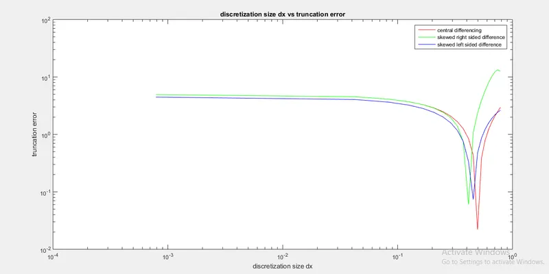
CONCLUSION:

As seen from the plot, Central differencing scheme the absolute error is very less when compared to other skewed schemes (skewed right sided and skewed left sided), as central difference uses information from both sides from the point of consideration to provide with an approximate and accurate value

Whereas skewed right sided and skewed left sided scheme uses information from one side i.e., either from right or left side end, from the point of consideration to provide with an approximate and less accurate value when compared to central difference scheme.

Why a skewed scheme is useful?

The system which doesn’t contain sufficient information on both side of the point of interest. In such cases we cannot use central differencing scheme so skewed scheme is useful in such cases.

What can a skewed scheme do that a CD scheme cannot?

Central Difference Scheme cannot not be employed at the boundary nodes due to unavailability of right and left nodes at the same time. In such cases the skewed differencing scheme is used.