Week 5.1 - Mid term project - Solving the steady and unsteady 2D heat conduction problem

AIM:

To solve the 2D heat conduction equation for steady and transient state by using the iterative techniques such as Jacobi, Gauss Seidel and Successive over relaxation method.

THEORY:

Heat conduction is defined as the process by which heat is transferred from the hotter end to the colder end of the object.

2-D heat conduction equation or ‘Transient’ heat conduction equation represented as:

`∂T/∂t+ α ((∂^2 T)/(∂x^2 )+(∂^2 T)/(∂y^2 ))=0`

Similarly, ‘Steady’ state heat conduction equation represented as:

`((∂^2 T)/(∂x^2 )+(∂^2 T)/(∂y^2 ))=0`

These equations above are partial differential equations, hence numerical discretization techniques can be used to solve these equations using the numerical analysis.

To solve by numerical discretization, assuming:

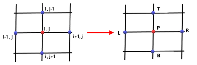
Where

T_P = T_i,j = Current point

T_L = T_i-1,j = Left hand side point

T_R = T_i+1,j = Left hand side point

T_B = T_i,j-1 = Bottom point

T_T = T_i,j+1 = Top point

Steady State heat conduction equation:

Steady state is where the fluid properties does not change with respect to time.

`((∂^2 T)/(∂x^2 )+(∂^2 T)/(∂y^2 ))=0`

Discretization:

`(∂^2 T)/(∂x^2 )= (T_(i-1,j) - 〖2*T〗_(i,j) + T_(i+1,j))/(Δx^2 )`

`(∂^2 T)/(∂y^2 )= (T_(i,j-1) - 〖2*T〗_(i,j) + T_(i,j+1))/(Δy^2 )`

For simplicity, subscripts are replaced as shown in above diagram:

`(T_L^n 〖- 2 . T〗_P^n + T_R^n)/〖Δx〗^2 + (T_T^n 〖 - 2 . T〗_P^n + T_B^n)/〖Δy〗^2 = 0`

Consider

`〖Δx〗^2/(2 . (〖Δx〗^2+ 〖Δy〗^2 ) )=k1`

`〖Δy〗^2/(2 . (〖Δx〗^2+ 〖Δy〗^2 ) )=k2`

For simplicity, subscripts are replaced as shown in above diagram

Jacobi Method:

In Jacobi method the value of the variables is not modified until next iteration.

`T_P^(n+1)= k1 . (T_L^n+ T_R^n ) +k2 . (T_T^n+ T_B^n )`

MATLAB Code:

close all 
clear all
clc 

% Steady state heat conduction 
% d^2*T/dx^2 + d^2*T/dy^2 = 0

% Defining input parameters 
% number of grid points along x and y direction
nx = 10;
ny = nx; 

% Creating a 2D mesh 
x = linspace(0,1,nx);
y = linspace(0,1,ny);
dx = x(2)-x(1);
dy = y(2)-y(1); 

% Absolute error criteria > tolerance
error = 9e9;
tol = 1e-4;


% Defining Boundary conditions
T_L = 400;
T_T = 600;
T_R = 800;
T_B = 900;

T = 300*ones(nx,ny);

T(2:ny - 1, 1)  = T_L;
T(2:ny - 1, nx) = T_R;
T(1, 2:nx - 1)  = T_T;
T(ny, 2:nx - 1) = T_B;

% Edge Refinement
T(1,1) = (T_T + T_L)/2;
T(nx,ny) = (T_R + T_B)/2;
T(1,ny) = (T_T + T_R)/2;
T(nx,1) = (T_L + T_B)/2;

% Assigning orginal values to T
T_intial = T;
T_old = T;

% Selection of the iterative solver method
iterative_solver = 1;

% Jacobi Iteration
if iterative_solver == 1
    jacobi_iteration = 1;
    
    while(error > tol)
        
        for i = 2:nx - 1
            
            for j = 2:ny - 1
                T(i,j) = 0.25*(T_old(i-1,j) + T_old(i+1,j) + T_old(i,j-1) + T_old(i,j+1));
            end
            
        end
        
        error = max(max(abs(T_old - T)));
        T_old = T;
        jacobi_iteration = jacobi_iteration + 1;  
        
    end
end

%Plotting
figure(1)
contourf(x,y,T)
clabel(contourf(x,y,T))
colormap(jet)
set(gca, 'ydir', 'reverse')
xlabel('X-Axis')
ylabel('Y-Axis')
title(sprintf('No. of Jacobi_Iterations = %d', jacobi_iteration));
pause(0.03);

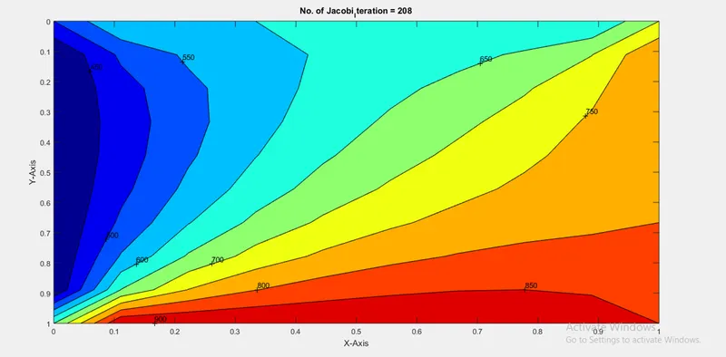
Output:

Gauss-Siedel Method:

In Gauss-Seidel method the value of the variables are modified as soon as new value is evaluated.

`T_P^(n+1)= k1 . (T_L^(n+1)+ T_R^(n+1) ) +k2 . (T_T^(n+1)+ T_B^(n+1) )`

MATLAB Code:

close all 
clear all
clc 

% Steady state heat conduction 
% d^2*T/dx^2 + d^2*T/dy^2 = 0

% Defining input parameters 
% number of grid points along x and y direction
nx = 10;
ny = nx; 

% Creating a 2D mesh 
x = linspace(0,1,nx);
y = linspace(0,1,ny);
dx = x(2)-x(1);
dy = y(2)-y(1); 

% Absolute error criteria > tolerance
error = 9e9;
tol = 1e-4;

% Defining Boundary conditions
T_L = 400;
T_T = 600;
T_R = 800;
T_B = 900;

T = 300*ones(nx,ny);

T(2:ny - 1, 1)  = T_L;
T(2:ny - 1, nx) = T_R;
T(1, 2:nx - 1)  = T_T;
T(ny, 2:nx - 1) = T_B;

% Edge Refinement
T(1,1) = (T_T + T_L)/2;
T(nx,ny) = (T_R + T_B)/2;
T(1,ny) = (T_T + T_R)/2;
T(nx,1) = (T_L + T_B)/2;

% Assigning orginal values to T
T_intial = T;
T_old = T;

% Selection of the iterative solver method
iterative_solver = 2;

% Gauss-Siedal Iteration
if iterative_solver == 2
    Gauss_seidel_iteration = 1;
    
    while(error > tol)
        
        for i = 2:nx - 1
            
            for j = 2:ny - 1
                T(i,j) = 0.25*(T(i-1,j) + T_old(i+1,j) + T(i,j-1) + T_old(i,j+1));
            end
            
        end
        
        error = max(max(abs(T_old - T)));
        T_old = T;
        Gauss_seidel_iteration = Gauss_seidel_iteration + 1;  
        
    end
end

%Plotting
figure(1)
contourf(x,y,T)
clabel(contourf(x,y,T))
colormap(jet)
set(gca, 'ydir', 'reverse')
xlabel('X-Axis')
ylabel('Y-Axis')
title(sprintf('No. of Gauss-Seidel_Iteration = %d', Gauss_seidel_iteration));
pause(0.03);

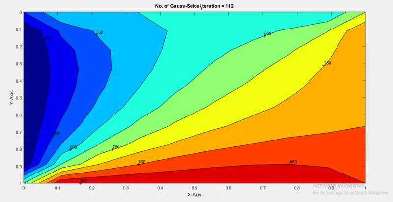
Output:

Successive over-relaxation Method:

Successive over-relaxation (SOR) is a variant of the Gauss–Seidel method for solving a linear system of equations, relaxation factor is used which helps in increasing the convergence rate.

`T_P^(n+1)=T_P^n .(1-ω)+ω .( k1 . (T_L^(n+1)+ T_R^(n+1) ) +k2 . (T_T^(n+1)+ T_B^(n+1) ))`

MATLAB Code:

close all 
clear all
clc 

% Steady state heat conduction 
% d^2*T/dx^2 + d^2*T/dy^2 = 0

% Defining input parameters 
% number of grid points along x and y direction
nx = 10;
ny = nx; 

% Creating a 2D mesh 
x = linspace(0,1,nx);
y = linspace(0,1,ny);
dx = x(2)-x(1);
dy = y(2)-y(1); 

% Absolute error criteria > tolerance
error = 9e9;
tol = 1e-4;
omega = 1.2;

% Defining Boundary conditions
T_L = 400;
T_T = 600;
T_R = 800;
T_B = 900;

T = 300*ones(nx,ny);

T(2:ny - 1, 1)  = T_L;
T(2:ny - 1, nx) = T_R;
T(1, 2:nx - 1)  = T_T;
T(ny, 2:nx - 1) = T_B;

% Edge Refinement
T(1,1) = (T_T + T_L)/2;
T(nx,ny) = (T_R + T_B)/2;
T(1,ny) = (T_T + T_R)/2;
T(nx,1) = (T_L + T_B)/2;

% Assigning orginal values to T
T_intial = T;
T_old = T;

% Selection of the iterative solver method
iterative_solver = 3;

% Successive Over_Relaxation Iteration
if iterative_solver == 3
    Successive_Over_Relaxation_iteration = 1;
    
    while(error > tol)
        
        for i = 2:nx - 1
            
            for j = 2:ny - 1
                T(i,j) = omega*(0.25*(T(i-1,j) + T_old(i+1,j) + T(i,j-1) + T_old(i,j+1))) + (1 - omega)*T_old(i,j);
            end
            
        end
        
        error = max(max(abs(T_old - T)));
        T_old = T;
        Successive_Over_Relaxation_iteration = Successive_Over_Relaxation_iteration + 1;  
        
    end
end

%Plotting
figure(1)
contourf(x,y,T)
clabel(contourf(x,y,T))
colormap(jet)
set(gca, 'ydir', 'reverse')
xlabel('X-Axis')
ylabel('Y-Axis')
title(sprintf('No. of Successive Over-Relaxation_Iteration = %d', Successive_Over_Relaxation_iteration));
pause(0.03);

Output:

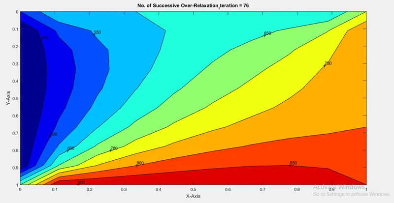
It can be concluded that the number of iteration required is least in SOR method. The maximum number of iteration is seen in jacobi method. So, the trend in terms of the number of iteration for convergence is:

Jacobi method > Gauss-siedel method > SOR method.

Transient heat conduction equation:

Unsteady or Transient state is where the fluid properties change with respect to time.

Time derivative `∂T/∂t`in equation is solved using forward time marching scheme.

`(T_(i,j)^(n+1)- T_(i,j)^n)/Δt`

Since, right hand side is elliptic in nature equation is solved using central difference scheme

`(∂^2 T)/(∂x^2 )= (T_(i-1,j) - 〖2*T〗_(i,j) + T_(i+1,j))/(Δx^2 )`

`(∂^2 T)/(∂y^2 )= (T_(i,j-1) - 〖2*T〗_(i,j) + T_(i,j+1))/(Δy^2 )`

For simplicity, subscripts are replaced as shown in above diagram

Explicit Form:

When a direct computation is made for an unknown quantity in terms of known quantity.

Derivative terms computed at the previous time step n, so the values at RHS are known.

`(T_P^(n+1) - T_P^n)/Δt= α .((T_L^n 〖- 2 . T〗_P^n + T_R^n)/〖Δx〗^2 + (T_T^n 〖 - 2 . T〗_P^n + T_B^n)/〖Δy〗^2 )`

Rearranging

`T_P^(n+1)= T_P^n+ α .Δt .((T_L^n 〖- 2 . T〗_P^n + T_R^n)/〖Δx〗^2 + (T_T^n 〖 - 2 . T〗_P^n + T_B^n)/〖Δy〗^2 )`

Consider

`(α .Δt)/〖Δx〗^2 =k1`

`(α .Δt)/〖Δy〗^2 =k2`

Substituting and rearranging values in above equation we get

`T_P^(n+1)= T_P^n .(1-2 .k1-2 .k2)+k1 .(T_L^n+ T_R^n )+ k1 .(T_T^n+ T_B^n )`

MATLAB Code:

close all
clear all
clc

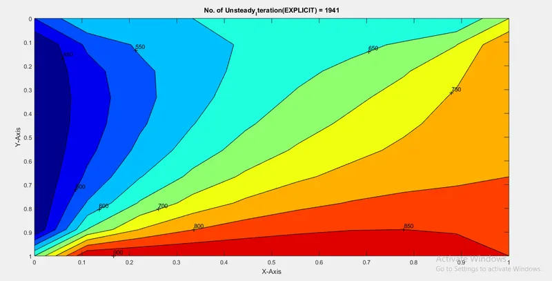
% Unsteady state 2D heat conduction equation (EXPLICIT SCHEME)
% dT/dt + α*(d^2*T/dx^2 + d^2*T/dy^2) = 0

% Definning input Parameters
% Number of grid points along x and y direction
nx = 10;
ny = nx;
nt = 1400;

% Creating a 2D mesh 
x = linspace(0,1,nx);
y = linspace(0,1,ny);
dx = x(2) - x(1);
dy = dx;

% Absolute error criteria > tolerance
error = 9e9;
tol = 1e-4;
dt = 1e-3;
omega = 1.1;

% Defining Boundary conditions
T_L = 400;
T_T = 600;
T_R = 800;
T_B = 900;

T = 300*ones(nx,ny);

T(2:ny - 1, 1)  = T_L;
T(2:ny - 1, nx) = T_R;
T(1, 2:nx - 1)  = T_T;
T(ny, 2:nx - 1) = T_B;

% Edge Refinement
T(1,1) = (T_T + T_L)/2;
T(nx,ny) = (T_R + T_B)/2;
T(1,ny) = (T_T + T_R)/2;
T(nx,1) = (T_L + T_B)/2;

%Assigning orginal values to T
T_intial = T;
T_old = T;


%Calculation of 2D steady heat conduction EQUATION by Successive over-relaxation method
iterative_solver = 1;
k1 = 1.1*(dt/(dx^2));
k2 = 1.1*(dt/(dy^2));

if iterative_solver == 1
    Steady_Explicit = 1;
    for k = 1:nt
        error = 1; 
    
        while(error > tol)
        
            for i = 2:nx - 1
            
                for j = 2:ny - 1
                    Term_1 = T_old(i,j);
                    Term_2 = k1*(T_old(i+1,j) - 2*T_old(i,j) + (T_old(i-1,j)));
                    Term_3 = k2*(T_old(i,j+1) - 2*T_old(i,j) + T_old(i,j-1));
                    T(i,j) = Term_1 + Term_2 + Term_3;
                end
            
            end
        
            error = max(max(abs(T_old - T)));
            T_old = T;
            Steady_Explicit = Steady_Explicit + 1;  
        
        end
    end
end

%Plotting
figure(1)
contourf(x,y,T)
clabel(contourf(x,y,T))
colormap(jet)
set(gca, 'ydir', 'reverse')
xlabel('X-Axis')
ylabel('Y-Axis')
title(sprintf('No. of Unsteady_Iteration(EXPLICIT) = %d', Steady_Explicit));
pause(0.03);

Output:

Implicit Form:

When a computation is made for dependent variable are defined by set of equations and a matrix is involved to find the unknown variable.

Derivative terms computed at the current time step n+1, so the values at RHS are unknown.

`(T_P^(n+1) - T_P^n)/Δt= α .((T_L^(n+1) 〖- 2 . T〗_P^(n+1) + T_R^(n+1))/〖Δx〗^2 + (T_T^(n+1) 〖 - 2 . T〗_P^(n+1) + T_B^(n+1))/〖Δy〗^2 )`

Rearranging

`T_P^(n+1)= T_P^n+ α .Δt .((T_L^(n+1) 〖- 2 . T〗_P^(n+1) + T_R^(n+1))/〖Δx〗^2 + (T_T^(n+1) 〖 - 2 . T〗_P^(n+1) + T_B^(n+1))/〖Δy〗^2 )`

Consider

`(α .Δt)/〖Δx〗^2 =k1`

`(α .Δt)/〖Δy〗^2 =k2`

Substituting and rearranging values in above equation we get

`T_P^(n+1)= ( T_P^n + k1 . (T_L^(n+1)+ T_R^(n+1) ) + k2 . (T_T^(n+1)+ T_B^(n+1) ))/(1 + 2 . k1+ 2 . k2)`

For implicit form the RHS is still unknown, to solve it directly could be challenging, using iterative solvers, iterative solver starting with initial guess and keep iterating it until the residual error comes below a specified limit.

Jacobi Method:

In Jacobi method the value of the variables is not modified until next iteration.

`T_P^(n+1)= ( T_P^n + k1 . (T_L^n+ T_R^n ) + k2 . (T_T^n+ T_B^n ))/(1 + 2 . k1+ 2 . k2)`

MATLAB Code:

close all
clear all
clc

% Unsteady state 2D heat conduction equation (IMPLICIT SCHEME)
% dT/dt + α*(d^2*T/dx^2 + d^2*T/dy^2) = 0

% Input Parameters
% Number of grid points along x and y direction
nx = 10;
ny = nx;
nt = 1400;

% Creating a 2D mesh 
x = linspace(0,1,nx);
y = linspace(0,1,ny);
dx = x(2) - x(1);
dy = dx;

%Absolute error criteria > tolerance
error = 9e9;
tol = 1e-4;
dt = 1e-3;

%Defining Boundary conditions
T_L = 400;
T_T = 600;
T_R = 800;
T_B = 900;

T = 300*ones(nx,ny);

T(2:ny - 1, 1)  = T_L;
T(2:ny - 1, nx) = T_R;
T(1, 2:nx - 1)  = T_T;
T(ny, 2:nx - 1) = T_B;

% Edge Refinement
T(1,1) = (T_T + T_L)/2;
T(nx,ny) = (T_R + T_B)/2;
T(1,ny) = (T_T + T_R)/2;
T(nx,1) = (T_L + T_B)/2;

% Assigning orginal values to T
T_old = T;
T_intial = T;

%Calculation of 2D steady heat conduction EQUATION by Successive over-relaxation method
k1 = 1.1*(dt/(dx^2));
k2 = 1.1*(dt/(dy^2));

Jacobi_iteration = 1;
for k = 1:nt
    error = 9e9; 
    
    while(error > tol)
        
        for i = 2:nx - 1
            
            for j = 2:ny - 1
                    
                Term_1 = 1/(1 + (2*k1) + (2*k2));
                Term_2 = k1*Term_1;
                Term_3 = k2*Term_1;
                H = (T_old(i-1,j)) + (T_old(i+1,j));
                V = (T_old(i,j+1)) + (T_old(i,j-1));
                    
                T(i,j) = (T_intial(i,j)*Term_1) + (H*Term_2) + (V*Term_3);
   
            end
            
        end
        
        error = max(max(abs(T_old - T)));
        T_old = T;
        Jacobi_iteration = Jacobi_iteration + 1;  
        
    end
    
    T_intial = T;
    
    %Plotting
    figure(1)
    contourf(x,y,T)
    clabel(contourf(x,y,T))
    colormap(jet)
    set(gca, 'ydir', 'reverse')
    xlabel('X-Axis')
    ylabel('Y-Axis')
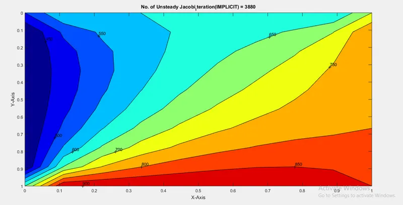
    title(sprintf('No. of Unsteady Jacobi_Iteration(IMPLICIT) = %d', Jacobi_iteration));
    pause(0.03)
end

Output:

Gauss-Siedel Method:

In Gauss-Seidel method the value of the variables are modified as soon as new value is evaluated.

`T_P^(n+1)= ( T_P^n + k1 . (T_L^(n+1)+ T_R^n ) + k2 . (T_T^n+ T_B^(n+1) ))/(1 + 2 . k1+ 2 . k2)`

MATLAB Code:

close all
clear all
clc

% Unsteady state 2D heat conduction equation (IMPLICIT SCHEME)
% dT/dt + α*(d^2*T/dx^2 + d^2*T/dy^2) = 0

% Input Parameters
% Number of grid points along x and y direction
nx = 10;
ny = nx;
nt = 1400;

% Creating a 2D mesh 
x = linspace(0,1,nx);
y = linspace(0,1,ny);
dx = x(2) - x(1);
dy = dx;

%Absolute error criteria > tolerance
error = 9e9;
tol = 1e-4;
dt = 1e-3;

%Defining Boundary conditions
T_L = 400;
T_T = 600;
T_R = 800;
T_B = 900;

T = 300*ones(nx,ny);

T(2:ny - 1, 1)  = T_L;
T(2:ny - 1, nx) = T_R;
T(1, 2:nx - 1)  = T_T;
T(ny, 2:nx - 1) = T_B;

% Edge Refinement
T(1,1) = (T_T + T_L)/2;
T(nx,ny) = (T_R + T_B)/2;
T(1,ny) = (T_T + T_R)/2;
T(nx,1) = (T_L + T_B)/2;

% Assigning orginal values to T
T_old = T;
T_intial = T;

%Calculation of 2D steady heat conduction EQUATION by Successive over-relaxation method
k1 = 1.1*(dt/(dx^2));
k2 = 1.1*(dt/(dy^2));

Gauss_Seidel_iteration = 1;
for k = 1:nt
    error = 9e9; 
    
    while(error > tol)
        
        for i = 2:nx - 1
            
            for j = 2:ny - 1
                    
                Term_1 = 1/(1 + (2*k1) + (2*k2));
                Term_2 = k1*Term_1;
                Term_3 = k2*Term_1;
                H = (T(i-1,j)) + (T_old(i+1,j));
                V = (T(i,j+1)) + (T_old(i,j-1));
                    
                T(i,j) = (T_intial(i,j)*Term_1) + (H*Term_2) + (V*Term_3);
   
            end
            
        end
        
        error = max(max(abs(T_old - T)));
        T_old = T;
        Gauss_Seidel_iteration = Gauss_Seidel_iteration + 1;  
        
    end
    
    T_intial = T;
    
    %Plotting
    figure(1)
    contourf(x,y,T)
    clabel(contourf(x,y,T))
    colormap(jet)
    set(gca, 'ydir', 'reverse')
    xlabel('X-Axis')
    ylabel('Y-Axis')
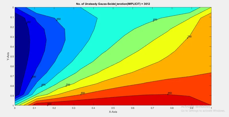
    title(sprintf('No. of Unsteady Gauss-Seidel_Iteration(IMPLICIT) = %d', Gauss_Seidel_iteration));
    pause(0.03)
end

Output:

Successive over-relaxation Method:

Successive over-relaxation (SOR) is a variant of the Gauss–Seidel method for solving a linear system of equations, relaxation factor is used which helps in increasing the convergence rate.

`T_P^(n+1)=T_P^n .(1-ω)+ ω . (( T_P^n + k1 . (T_L^n+ T_R^n ) + k2 . (T_T^n+ T_B^n ))/(1 + 2 . k1+ 2 . k2))`

MATLAB Code:

close all
clear all
clc

% Unsteady state 2D heat conduction equation (IMPLICIT SCHEME)
% dT/dt + α*(d^2*T/dx^2 + d^2*T/dy^2) = 0

% Input Parameters
% Number of grid points along x and y direction
nx = 10;
ny = nx;
nt = 1400;

% Creating a 2D mesh 
x = linspace(0,1,nx);
y = linspace(0,1,ny);
dx = x(2) - x(1);
dy = dx;

%Absolute error criteria > tolerance
error = 9e9;
tol = 1e-4;
dt = 1e-3;
omega = 1.1;

%Defining Boundary conditions
T_L = 400;
T_T = 600;
T_R = 800;
T_B = 900;

T = 300*ones(nx,ny);

T(2:ny - 1, 1)  = T_L;
T(2:ny - 1, nx) = T_R;
T(1, 2:nx - 1)  = T_T;
T(ny, 2:nx - 1) = T_B;

% Edge Refinement
T(1,1) = (T_T + T_L)/2;
T(nx,ny) = (T_R + T_B)/2;
T(1,ny) = (T_T + T_R)/2;
T(nx,1) = (T_L + T_B)/2;

% Assigning orginal values to T
T_old = T;
T_intial = T;
T_end = T;

%Calculation of 2D steady heat conduction EQUATION by Successive over-relaxation method
k1 = 1.1*(dt/(dx^2));
k2 = 1.1*(dt/(dy^2));

Successive_over_relaxation_iteration = 1;
for k = 1:nt
    error = 9e9; 
    
    while(error > tol)
        
        for i = 2:nx - 1
            
            for j = 2:ny - 1
                    
                Term_1 = 1/(1 + (2*k1) + (2*k2));
                Term_2 = k1*Term_1;
                Term_3 = k2*Term_1;
                H = (T(i-1,j)) + (T_old(i+1,j));
                V = (T(i,j+1)) + (T_old(i,j-1));
                    
                T(i,j) = (T_intial(i,j)*Term_1) + (H*Term_2) + (V*Term_3);
                T_end(i,j) = ((1-omega)*T_old(i,j)) + (T(i,j)*omega);
                
            end
            
        end
        
        error = max(max(abs(T_old - T)));
        T_old = T_end;
        Successive_over_relaxation_iteration = Successive_over_relaxation_iteration + 1;  
        
    end
    
    T_intial = T_end;
    
    %Plotting
    figure(1)
    contourf(x,y,T)
    clabel(contourf(x,y,T))
    colormap(jet)
    set(gca, 'ydir', 'reverse')
    xlabel('X-Axis')
    ylabel('Y-Axis')
    title(sprintf('No. of Unsteady SOR_Iteration(IMPLICIT) = %d', Successive_over_relaxation_iteration));
    pause(0.03)
end

Output:

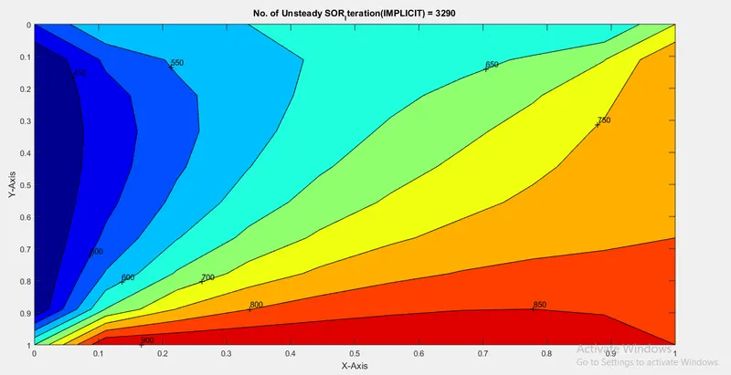
It can be concluded that the number of iteration required is least in SOR method. The maximum number of iteration is seen in jacobi method. So, the trend in terms of the number of iteration for convergence is:

Jacobi method > Gauss-siedel method > SOR method.