Week 7 - Simulation of a 1D Super-sonic nozzle flow simulation using Macormack Method
GOVERNING EQUATION :
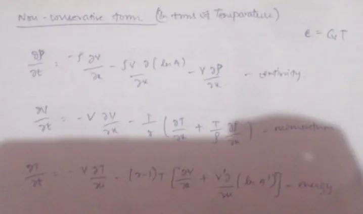
NON-CONSERVATION :
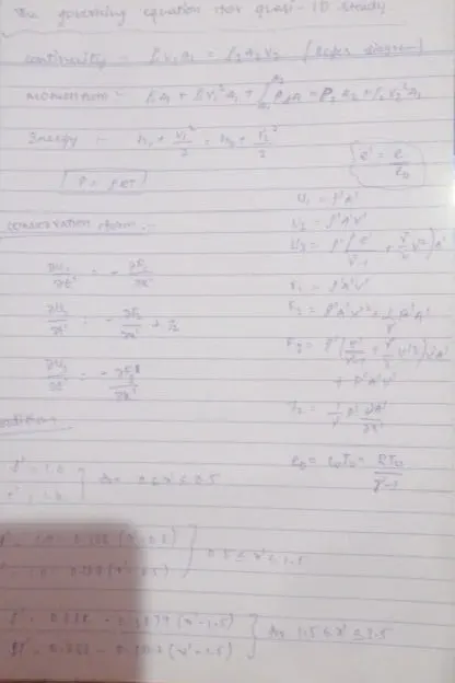
CONSERVATION :
MATHLAB CODE :
close all
clear all
clc


n=61;
x=linspace(0,3,n);
dx=x(2)-x(1);
rho=1-0.3146*x;
t=1-0.2314*x;
v=(0.1+1.09*x).*t.^0.5;
a=1+2.2*(x-1.5).^2;

nt=1400;
gamma=1.4;
dt=min(0.5.*dx./(sqrt(t)+v));

tic;
[v_n,rho_n,t_n,Mach_num_n,mass_flow_n,ctr_n,dt_n]= non_conservation(n,x,dx,rho,t,v,a,nt,gamma);
non_time=toc;

tic;
[v_c,rho_c,t_c,Mach_num_c,mass_flow_c,ctr_c,dt_c]= conservation(n,x,dx,nt,gamma) ;
cons_time=toc;

figure(7)
 plot(x,mass_flow_n);
 hold on;
 plot(x,mass_flow_c);
 xlabel('x\l');
 ylabel('mass flow rate');
 title('comparison of mass flow rate');
 legend('NON-Conservative','Conservative');


 time=[non_time cons_time];
 iter=[ctr_n ctr_c];
 x=[1 2];
 figure(9);
 grid on;

 subplot(2,1,1);
 bar(x,time);
 xlabel('1.NON-CONSERVATIVE APPROACH   2.CONSERVATIVE APPROCH');
 ylabel('time taken to attain steady state');
 title('time comparison of CONS. and NON-CONS. approach to attain steady state');

 subplot(2,1,2);
 bar(x,iter);
 xlabel('1.NON-CONSERVATIVE APPROACH   2.CONSERVATIVE APPROCH');
 ylabel('iter taken to attain steady state');
 title('iter comparison of CONS. and NON-CONS. approach to attain steady state');

function[v,rho,t,Mach_num,mass_flow,ctr,dt]= non_conservation(n,x,dx,rho,t,v,a,nt,gamma)

ctr=1;
cs=1;

for k=1:nt

  rho_old=rho;
  v_old=v;
  t_old=t;
  dt=min(0.5.*dx./(sqrt(t)+v));

 for i=2:n-1

  dvdx=(v(i+1)-v(i))/dx;
  drhodx=(rho(i+1)-rho(i))/dx;
  dtdx=(t(i+1)-t(i))/dx;
  dlogadx=(log(a(i+1))-log(a(i)))/dx;

  drhodt_p(i)= -rho(i)*dvdx-rho(i)*v(i)*dlogadx-v(i)*drhodx;
  dvdt_p(i)= -v(i)*dvdx-(1/gamma)*(dtdx+(t(i)/rho(i))*drhodx);
  dtdt_p(i)= -v(i)*dtdx-(gamma-1)*t(i)*(dvdx+v(i)*dlogadx);

  rho(i)=rho(i)+drhodt_p(i)*dt;
  v(i)=v(i)+dvdt_p(i)*dt;
  t(i)=t(i)+dtdt_p(i)*dt;
end

for i=2:n-1

  dvdx=(v(i)-v(i-1))/dx;
  drhodx=(rho(i)-rho(i-1))/dx;
  dtdx=(t(i)-t(i-1))/dx;
  dlogadx=(log(a(i))-log(a(i-1)))/dx;

  drhodt_c(i)= -rho(i)*dvdx-rho(i)*v(i)*dlogadx-v(i)*drhodx;
  dvdt_c(i)= -v(i)*dvdx-(1/gamma)*(dtdx+t(i)/rho(i)*drhodx);
  dtdt_c(i)= -v(i)*dtdx-(gamma-1)*t(i)*(dvdx+v(i)*dlogadx);

end
  drhodt_avg=0.5*(drhodt_p+drhodt_c);
  dvdt_avg=0.5*(dvdt_p+dvdt_c);
  dtdt_avg=0.5*(dtdt_p+dtdt_c);

  for j=2:n-1
    rho(j)=rho_old(j)+drhodt_avg(j)*dt;
    v(j)=v_old(j)+dvdt_avg(j)*dt;
    t(j)=t_old(j)+dtdt_avg(j)*dt;
  end
  #inlet
  v(1)=2*v(2)-v(3);
  #outlet
  v(n)=2*v(n-1)-v(n-2);
  rho(n)=2*rho(n-1)-rho(n-2);
  t(n)=2*t(n-1)-t(n-2);

 for i=1:n
  Mach_num(i)=v(i)/(sqrt(t(i)));
  mass_flow(i)=rho(i)*v(i)*a(i);
end

error1=max(abs(v-v_old));
error2=max(abs(rho-rho_old));
error3=max(abs(t-t_old));

rho_th(k) = rho(16);
t_th(k) = t(16);
Mach_num_th(k) = Mach_num(16);
v_th(k) = v(16);

% Mass Flow rate at different time steps
if(ctr==100 || ctr==300 || ctr==500 || ctr==700)
 figure(1);
 color=['g','b','r','*'];
 plot(x,mass_flow,color(cs),'linewidth',1);
 legend('100t','300t','500t','800t','location','bestoutside');
 title('mass flow rates at different time steps in non conservative form');
 xlabel('X/L');
 ylabel('mass flow rate');
 cs=cs+1;
 hold on;
 axis([0 3 0 2]);
 pause(0.001)
end


ctr=ctr+1;

end

figure(2);
grid on ;
subplot(4,1,1);
plot(v_th,'b');
title('variation of the Veloctity at throat w.r.t time');
xlabel('Time Iterations');
ylabel('Velocity');


subplot(4,1,2);
plot(rho_th,'g');
title('variation of the Density at throat w.r.t time');
xlabel('Time Iterations');
ylabel('Density');


subplot(4,1,3);
plot(t_th,'r');
title('variation of the Temperature at throat w.r.t time');
xlabel('Time Iterations');
ylabel('Temperature');


subplot(4,1,4);
plot(Mach_num_th,'m');
title('variation of the Mach_num at throat w.r.t time');
xlabel('Time Iterations');
ylabel('Mach_num');

figure(3)
subplot(4,1,1)
plot(x,v)
title(sprintf('variation of Velocity wrt distance x at time step : %d ',ctr));
xlabel('X/l');
ylabel('V/a');

subplot(4,1,2)
plot(x,rho)
title(sprintf('variation of Density wrt distance x at time step : %d ',ctr));
xlabel('X/l');
ylabel('rho/rho_not');

subplot(4,1,3)
plot(x,t)
title(sprintf('variation of Temparature wrt distance x at time step : %d ',ctr));
xlabel('X/l');
ylabel('T/T_not');

subplot(4,1,4)
plot(x,Mach_num)
title(sprintf('variation of Mach number wrt distance x at time step : %d ',ctr));
xlabel('X/l');
ylabel('M');

end


function[v,rho,t,Mach_num,mass_flow,ctr,dt]= non_conservation(n,x,dx,rho,t,v,a,nt,gamma)

ctr=1;
cs=1;

for k=1:nt

  rho_old=rho;
  v_old=v;
  t_old=t;
  dt=min(0.5.*dx./(sqrt(t)+v));

 for i=2:n-1

  dvdx=(v(i+1)-v(i))/dx;
  drhodx=(rho(i+1)-rho(i))/dx;
  dtdx=(t(i+1)-t(i))/dx;
  dlogadx=(log(a(i+1))-log(a(i)))/dx;

  drhodt_p(i)= -rho(i)*dvdx-rho(i)*v(i)*dlogadx-v(i)*drhodx;
  dvdt_p(i)= -v(i)*dvdx-(1/gamma)*(dtdx+(t(i)/rho(i))*drhodx);
  dtdt_p(i)= -v(i)*dtdx-(gamma-1)*t(i)*(dvdx+v(i)*dlogadx);

  rho(i)=rho(i)+drhodt_p(i)*dt;
  v(i)=v(i)+dvdt_p(i)*dt;
  t(i)=t(i)+dtdt_p(i)*dt;
end

for i=2:n-1

  dvdx=(v(i)-v(i-1))/dx;
  drhodx=(rho(i)-rho(i-1))/dx;
  dtdx=(t(i)-t(i-1))/dx;
  dlogadx=(log(a(i))-log(a(i-1)))/dx;

  drhodt_c(i)= -rho(i)*dvdx-rho(i)*v(i)*dlogadx-v(i)*drhodx;
  dvdt_c(i)= -v(i)*dvdx-(1/gamma)*(dtdx+t(i)/rho(i)*drhodx);
  dtdt_c(i)= -v(i)*dtdx-(gamma-1)*t(i)*(dvdx+v(i)*dlogadx);

end
  drhodt_avg=0.5*(drhodt_p+drhodt_c);
  dvdt_avg=0.5*(dvdt_p+dvdt_c);
  dtdt_avg=0.5*(dtdt_p+dtdt_c);

  for j=2:n-1
    rho(j)=rho_old(j)+drhodt_avg(j)*dt;
    v(j)=v_old(j)+dvdt_avg(j)*dt;
    t(j)=t_old(j)+dtdt_avg(j)*dt;
  end
  #inlet
  v(1)=2*v(2)-v(3);
  #outlet
  v(n)=2*v(n-1)-v(n-2);
  rho(n)=2*rho(n-1)-rho(n-2);
  t(n)=2*t(n-1)-t(n-2);

 for i=1:n
  Mach_num(i)=v(i)/(sqrt(t(i)));
  mass_flow(i)=rho(i)*v(i)*a(i);
end

error1=max(abs(v-v_old));
error2=max(abs(rho-rho_old));
error3=max(abs(t-t_old));

rho_th(k) = rho(16);
t_th(k) = t(16);
Mach_num_th(k) = Mach_num(16);
v_th(k) = v(16);

% Mass Flow rate at different time steps
if(ctr==100 || ctr==300 || ctr==500 || ctr==700)
 figure(1);
 color=['g','b','r','*'];
 plot(x,mass_flow,color(cs),'linewidth',1);
 legend('100t','300t','500t','800t','location','bestoutside');
 title('mass flow rates at different time steps in non conservative form');
 xlabel('X/L');
 ylabel('mass flow rate');
 cs=cs+1;
 hold on;
 axis([0 3 0 2]);
 pause(0.001)
end


ctr=ctr+1;

end

figure(2);
grid on ;
subplot(4,1,1);
plot(v_th,'b');
title('variation of the Veloctity at throat w.r.t time');
xlabel('Time Iterations');
ylabel('Velocity');


subplot(4,1,2);
plot(rho_th,'g');
title('variation of the Density at throat w.r.t time');
xlabel('Time Iterations');
ylabel('Density');


subplot(4,1,3);
plot(t_th,'r');
title('variation of the Temperature at throat w.r.t time');
xlabel('Time Iterations');
ylabel('Temperature');


subplot(4,1,4);
plot(Mach_num_th,'m');
title('variation of the Mach_num at throat w.r.t time');
xlabel('Time Iterations');
ylabel('Mach_num');

figure(3)
subplot(4,1,1)
plot(x,v)
title(sprintf('variation of Velocity wrt distance x at time step : %d ',ctr));
xlabel('X/l');
ylabel('V/a');

subplot(4,1,2)
plot(x,rho)
title(sprintf('variation of Density wrt distance x at time step : %d ',ctr));
xlabel('X/l');
ylabel('rho/rho_not');

subplot(4,1,3)
plot(x,t)
title(sprintf('variation of Temparature wrt distance x at time step : %d ',ctr));
xlabel('X/l');
ylabel('T/T_not');

subplot(4,1,4)
plot(x,Mach_num)
title(sprintf('variation of Mach number wrt distance x at time step : %d ',ctr));
xlabel('X/l');
ylabel('M');

end
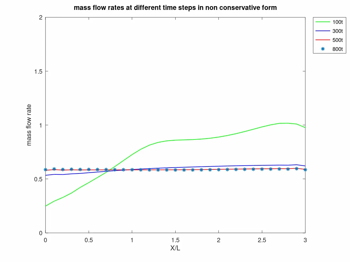
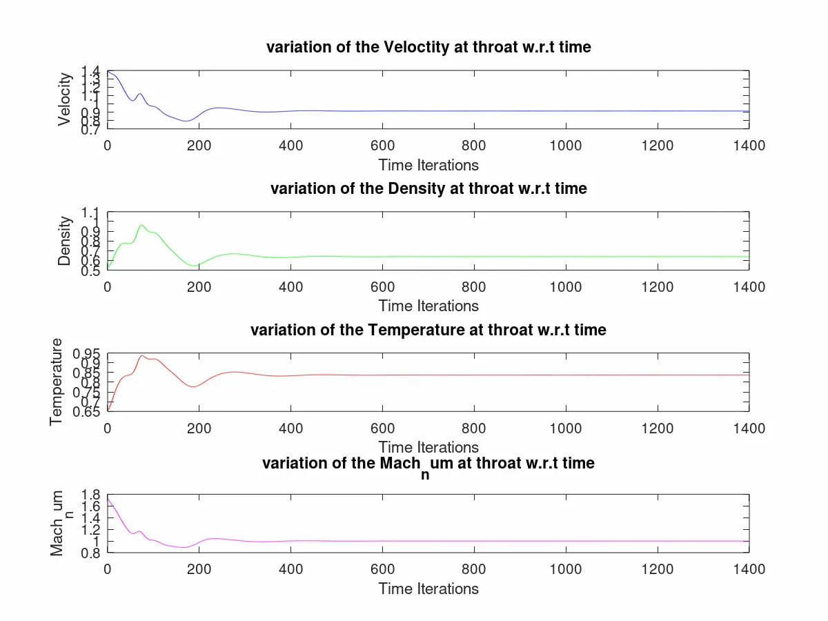
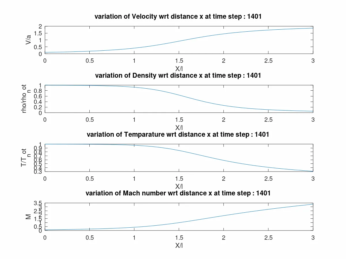
PLOTS FOR NON-CONSERVATION :
PLOTS FOR CONSERVATION :
COMPARISATION PLOT :
CONCLUSION :
GRID DEPENDANCY - The rho(16) value for 31 gird is 0.65237 whereas the rho(16) value for 61 grid is 0.63908.The v(16) value for 31 gird is 0.89691whereas the v(16) value for 61 grid is 0.91212.The t(16) value for 31 gird is 0.84103 whereas the t(16) value for 61 grid is 0.83555. from this it is conclusive that dx decreases with the increase in the grid points,But this produce some better accuracy.The value of the characterstics parameter are more closer to the exact value.
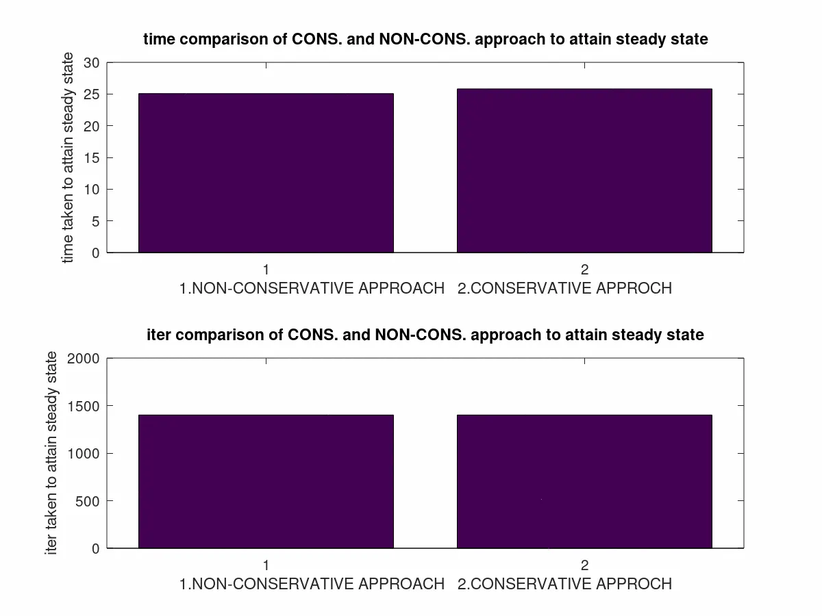
Total number of time taken is slighty more for conservative the compared to that of non-conservative 25.078 and 25.813.This is because the conservative form cannot be solved directly through the primitive form as it may lead to unstable solution.
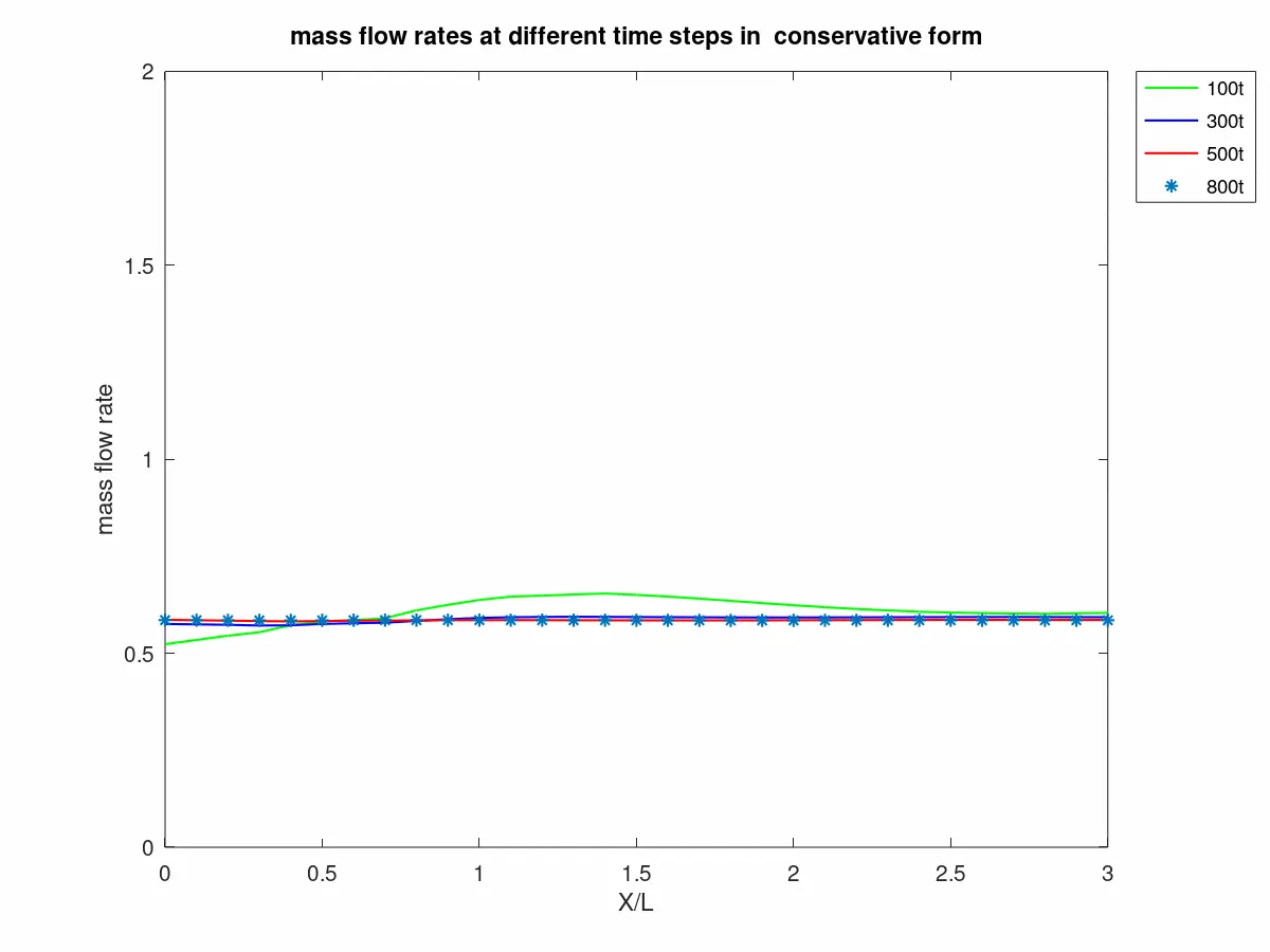
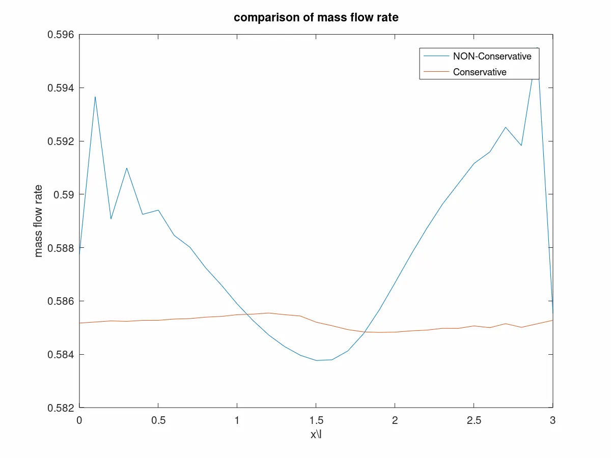
The non-conservative approach is slightly faster than that of the conservative form and the values are closer to that of the analytical solution from john D anderson book. In terms of mass flow rate the conservative form has an edge over the non-conservative form, As it is clear from the graph where the graph goes steady for the conservative form.
The results obtained from both the approaches are grid independent as there is no larger change in the output with the change in the grid points.
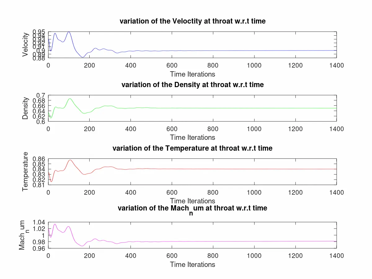
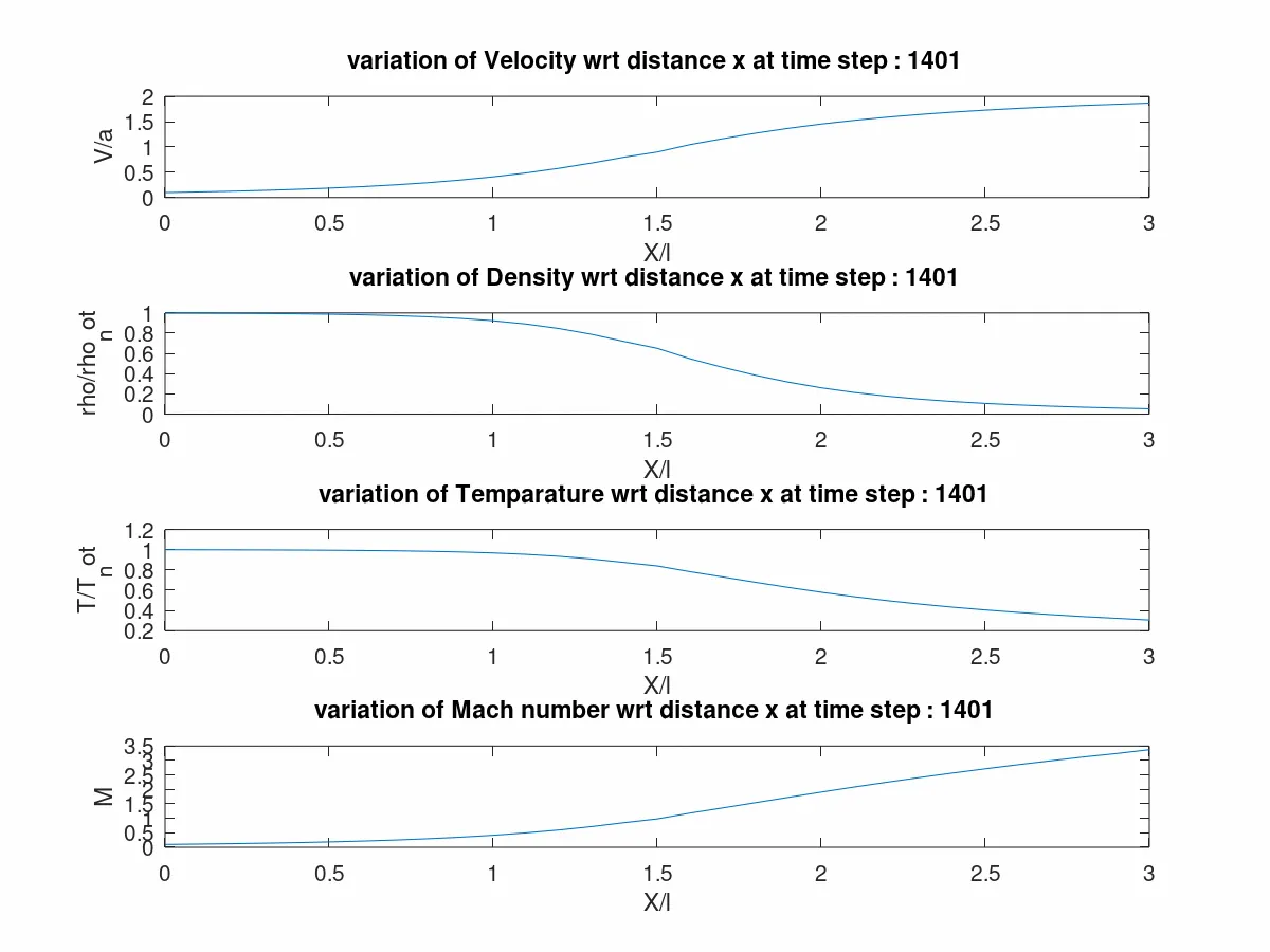
As it is a supersonic flow, the velocity and the Mach number tends to increases at the throat whereas density and temparature decreases at the throat.