Week 5 - Mid term project - Solving the steady and unsteady 2D heat conduction problem

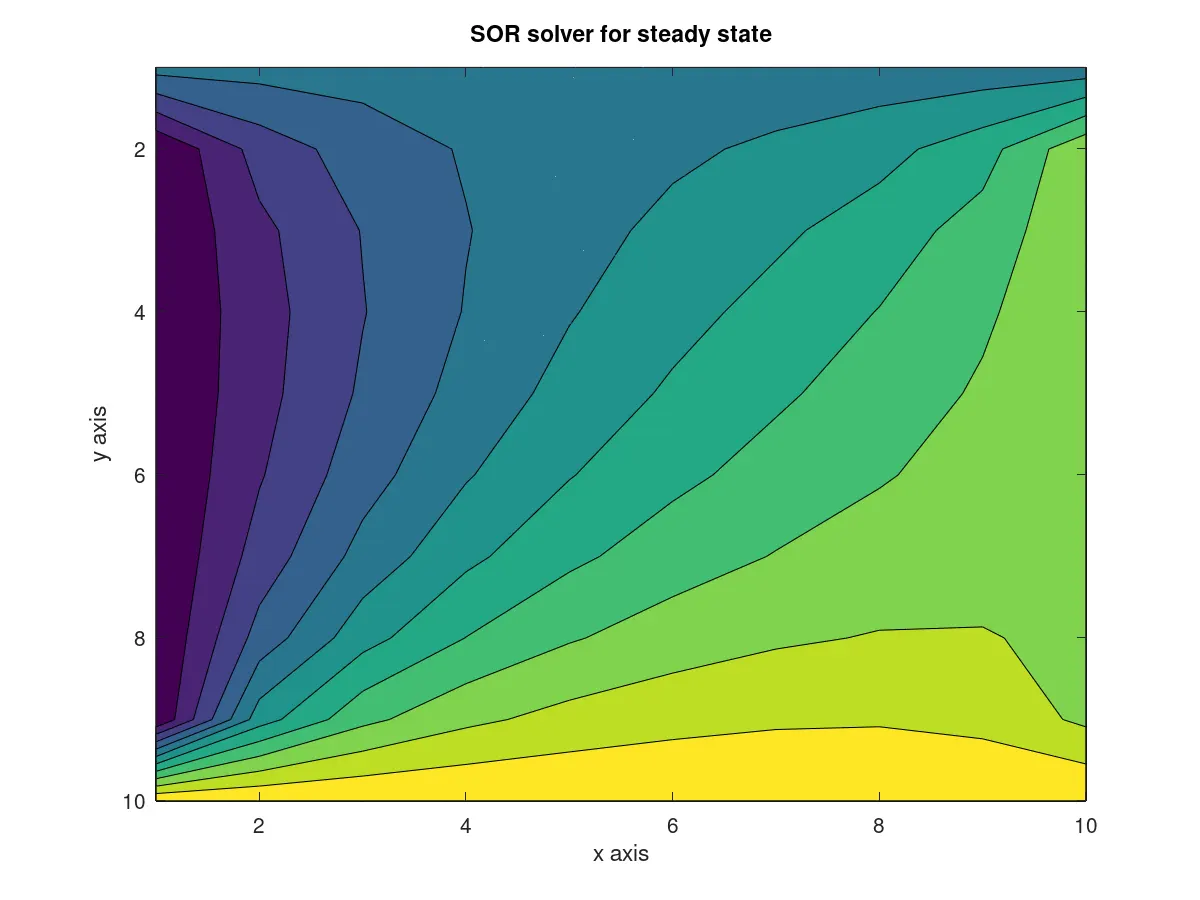
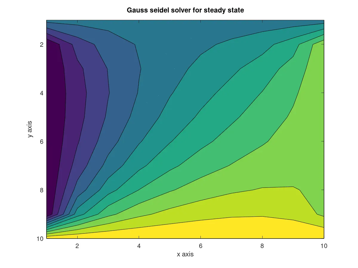
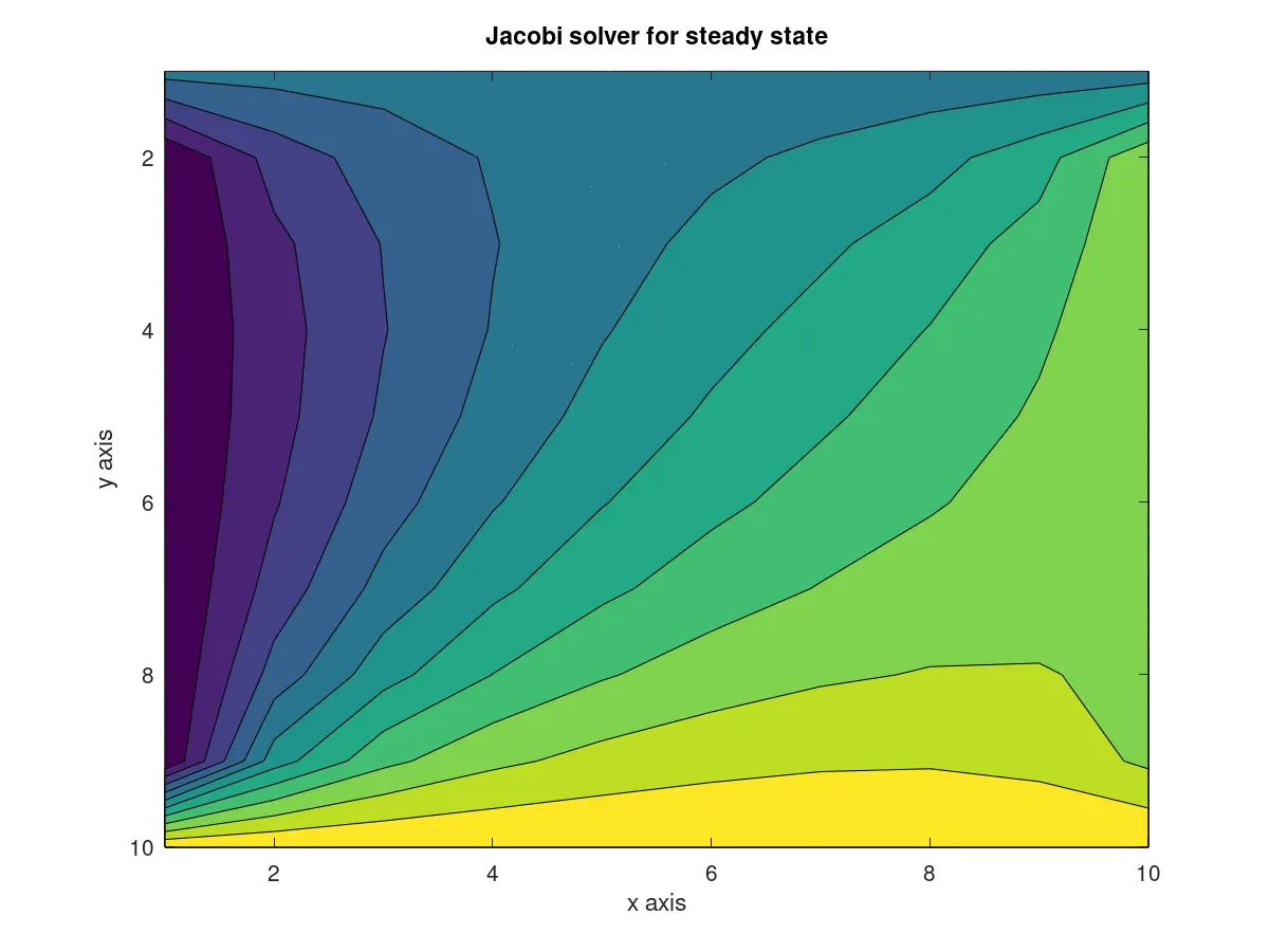
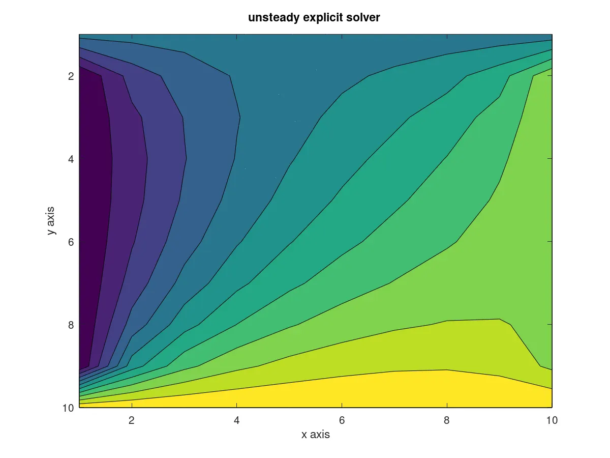
function T=sor(error,Tol,nx,ny,T_old,w,T)
while error > Tol
  for i=2:nx-1
    for j=2:ny-1
      
      Tgs(i,j)=(1/4)*(((T(i-1,j)+ T_old(i+1,j)))+ ((T(i,j-1)+T_old(i,j+1))));
      T(i,j)=(1-w)*T_old(i,j)+w*Tgs(i,j);
   end
  end
  error=max(max(abs(T_old - T)));
  T_old=T;
  contourf(T);
  axis ij;
  axis ij;
  pause(0.01)
  
end

function T=assig5_gaussseidel_sor(error,Tol,nx,ny,T_old,T)

while error > Tol
  for i=2:nx-1
    for j=2:ny-1
      
      T(i,j)=(1/4)*(((T(i-1,j)+ T_old(i+1,j)))+ ((T(i,j-1)+T_old(i,j+1))));
   end
  end
  error=max(max(abs(T_old - T)));
  T_old=T;
  contourf(T);
  axis ij;
  pause(0.01)
  
end

function T=assig5_gaussseidel_sor(error,Tol,nx,ny,T_old,T)

while error > Tol
  for i=2:nx-1
    for j=2:ny-1
      
      T(i,j)=(1/4)*(((T(i-1,j)+ T_old(i+1,j)))+ ((T(i,j-1)+T_old(i,j+1))));
   end
  end
  error=max(max(abs(T_old - T)));
  T_old=T;
  contourf(T);
  axis ij;
  pause(0.01)
  
end

function T=assig5_unsteady_explicit(nt,nx,ny,T,T_prev,k1,k2)

for k = 1:nt
  for i=2:nx-1;
    for j=2:ny-1;
      T(i,j)=T(i,j)+k1*(T_prev(i-1,j)-(2*T_prev(i,j))+T_prev(i+1,j))+k2*(T_prev(i,j-1)-(2*T_prev(i,j))+T_prev(i,j+1));
    end
  end
  T_prev = T;
  contourf(T);
  axis ij;
  pause(0.01)
end

function T=assig5_implicit_jacobi(nt,Tol,nx,ny,k1,k2,T_old,T,T_prev)


for nt=1:1400
    error = 1;
    while error > Tol
      for i=2:nx-1;
        for j=2:ny-1;
            term1=(1+(2*k1)+(2*k2))^-1;
            term2=k1*term1;
            term3=k2*term1;
            H=T_old(i-1,j)+T_old(i+1,j);
            V=T_old(i,j-1)+T_old(i,j+1);

          T(i,j)=(T_prev(i,j)*term1)+(term2*H)+(term3*V);
        end
      end
      error=max(T_old-T);
      T_old=T;
      
    end
    T_prev=T;
  end
  contourf(T);
  axis ij;

function T=assig5_implicit_gauss(nt,Tol,nx,ny,k1,k2,T_old,T,T_prev)


for nt=1:1400
    error = 1;
    while error > Tol
      for i=2:nx-1;
        for j=2:ny-1;
            term1=(1+(2*k1)+(2*k2))^-1;
            term2=k1*term1;
            term3=k2*term1;
            H=T(i-1,j)+T(i+1,j);
            V=T(i,j-1)+T(i,j+1);

          T(i,j)=(T_prev(i,j)*term1)+(term2*H)+(term3*V);
        end
      end
      error=max(T_old-T);
      T_old=T;
    end
    T_prev=T;
  end
  contourf(T);
  axis ij; 

function T=assig5_implicit_SOR(nt,Tol,nx,ny,k1,k2,T_old,T,T_prev,w);

for nt=1:1400
    error = 1;
    while error > Tol
      for i=2:nx-1;
        for j=2:ny-1;
            term1=(1+(2*k1)+(2*k2))^-1;
            term2=k1*term1;
            term3=k2*term1;
            H=T(i-1,j)+T(i+1,j);
            V=T(i,j-1)+T(i,j+1);

          Tgs(i,j)=(T_prev(i,j)*term1)+(term2*H)+(term3*V);
          T(i,j)=(1-w)*T_old(i,j)+w*((T_prev(i,j)*term1)+(term2*H)+(term3*V));
        end
      end
      error=max(T_old-T);
      T_old=T;
    end
    T_prev=T   ;
  end
  contourf(T);
  axis ij;

clear all 
close all 
clc 

nx = 10;
ny = 10;
x=linspace(0,1,nx);
y=linspace(0,1,ny);
dx = x(2)-x(1);
dy = y(2)-y(1);

T = 300*ones(nx,ny);
T(:,1)=400;
T(:,nx)=800;
T(1,:)=600;
T(ny,:)=900;
k=2*((nx^2+ny^2)/(nx^2*ny^2));
t = 2;
dt = 1e-3;
nt = t/dt;
alpha=1.4;
k1=alpha*(dt/dx^2);
k2=alpha*(dt/dy^2);
w=1.2;
T_prev = T;
T_old=T;
T_intial=T;
Tol=1e-4;
error=1;

figure 1
T_s=sor(error,Tol,nx,ny,T_old,w,T);
xlabel('x axis');
ylabel('y axis');
title('SOR solver for steady state'); 

figure 2
T_g=assig5_gaussseidel_sor(error,Tol,nx,ny,T_old,T);
xlabel('x axis');
ylabel('y axis');
title('Gauss seidel solver for steady state'); 
figure 3
T_jac=assig5jacobi(error,Tol,nx,ny,T_old,T);
xlabel('x axis');
ylabel('y axis');
title('Jacobi solver for steady state'); 
figure 4
T_us=assig5_unsteady_explicit(nt,nx,ny,T,T_prev,k1,k2);
xlabel('x axis');
ylabel('y axis');
title('unsteady explicit solver '); 
figure 5
T_j=assig5_implicit_jacobi(nt,Tol,nx,ny,k1,k2,T_old,T,T_prev);
xlabel('x axis');
ylabel('y axis');
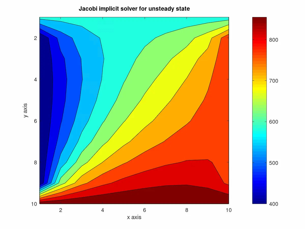
title('Jacobi implicit solver for unsteady state');
colorbar; 
colormap(jet);
figure 6
T_g=assig5_implicit_gauss(nt,Tol,nx,ny,k1,k2,T_old,T,T_prev);
xlabel('x axis');
ylabel('y axis');
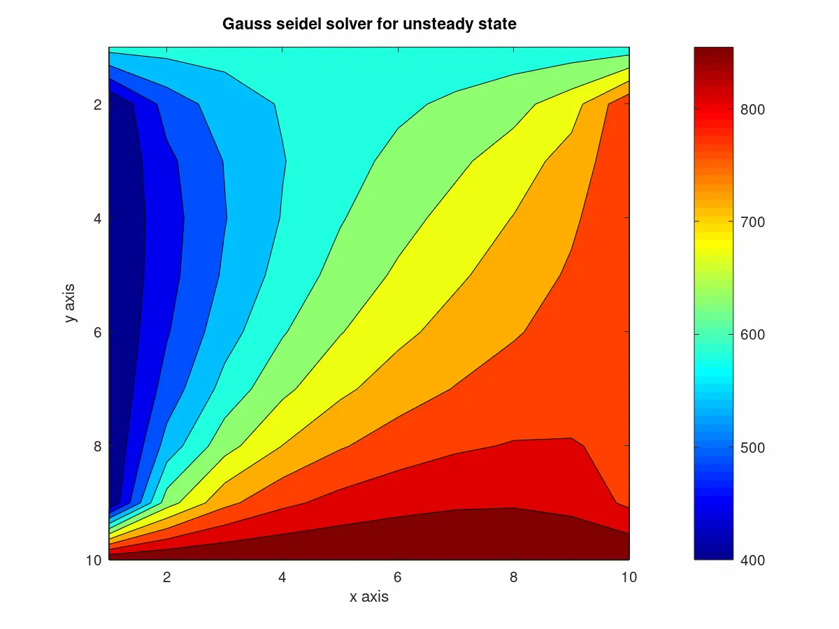
title('Gauss seidel solver for unsteady state'); 
colorbar;
colormap(jet);
figure 7
T_sor=assig5_implicit_SOR(nt,Tol,nx,ny,k1,k2,T_old,T,T_prev,w);
xlabel('x axis');
ylabel('y axis');
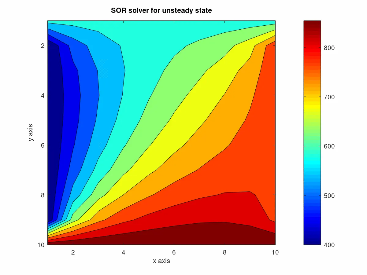
title('SOR solver for unsteady state'); 
colorbar;
colormap(jet);

RESULT :

For the steady state condition it has been solved using jacobi,gauss seidel, SOR. In the jacobi method the solution is obtaine only after all the grid point are calculated , whereas the gauss seidel and SOR works by updating the new values. And in the SOR the relaxtion factor is added to the temparature. Thus the time taken to obtain solution is faster with the SOR then gauss seidel then by jacobi.

In the unsteady explicit conditon , we use time marching method to bring the solution to the steady state .

Whereas implicit unsteady condition , we again use the jacobi,gauss seidel, SOR to solve with the time marching method . As the number of unknows are greater we need to use the iterative method to get the steady state solution. Since SOR is faster the iteration is lesser for SOR compared to others