Simulation of a 1D Super-sonic nozzle flow simulation using Macormack Method
Objective:
To solve the Quasi 1-D supersonic nozzle flow equation using the Macormack method in MATLAB.
To compare the variations in flow field variables in conservative and non-conservative forms of the equation.
To perform a grid dependency test.
Quasi 1-D Supersonic nozzle flow:
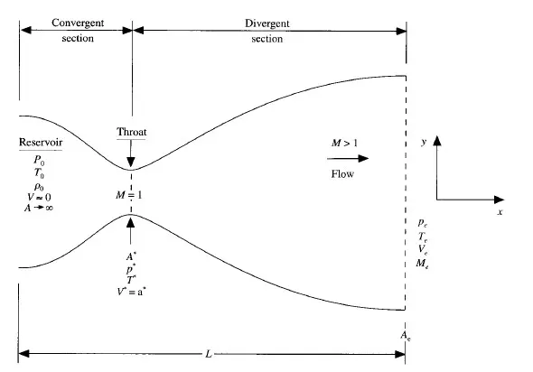
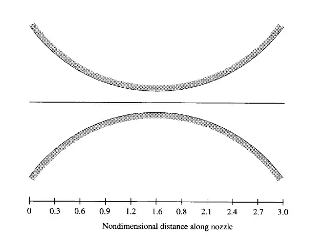
The flow analysis is to be carried out for a convergent-divergent nozzle as given below:
Procedure:
1. Creating the mesh
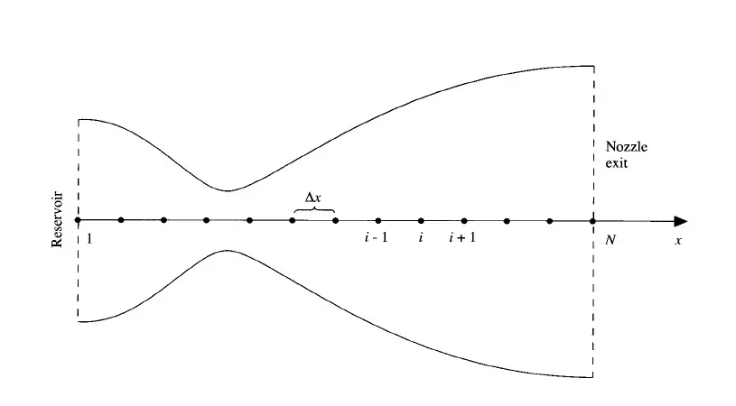
For the simplicity of the problem, flow is assumed to be 1-D along the X-axis.
Domain parameters:
Length = 3m
Number of grid points = 31
Distance between grids = 0.1m
2. Discretization
MacCormack method plays a major role and provides a time marching solution. The step used in this method is as follows.
MacCormack method:
Let the f(x) be the equation to be solved.
i) initial profile:
Before the calculation, the initial profile for all the flow field variables should be specified. The profile is as follows,
ii) Predictor step:
`((delf)/(delt))_p = (f(i+1)-f(i))/(Deltax)`
iii) solution update:
`f_p=f_(Initial)+((delf)/(delt))_p*Deltat`
`f_p` = Flow field variables calculated after the predictor step
`f_(Initial)` = Flow field variables at their initial profile
`Deltat` = Timestep size
iv) Corrector step:
`((delf)/(delt))_c = (f(i)-f(i-1))/(Deltax)`
After that find the average value
`((delf)/(delt))_(avg) =0.5*(((delf)/(delt))_p +((delf)/(delt))_c )`
v) Final solution update:
`f_(sol) = f_(Initial)+((delf)/(delt))_(avg)*(Deltat)`
`f_(sol)` = Final solution of the flow field variables for the first time step.
3.Solving equation:
a) Non-conservative form:
i) Continuity equation:
`(delrho')/(delt') = -rho'((delV')/(delx')) - rho'V'((del(lnA'))/(delx')) - V'((delrho')/(delx'))`
ii) Momentum equation:
`(delV')/(delt') = -V'((delV')/(delx')) - (1/gamma)((delT')/(delx')+(T')/(rho')((delrho')/(delx')))`
iii) Energy equation:
`(delT')/(delt') = -V'((delT')/(delx'))- (gamma-1)T'[(delV')/(delx') + V'(del(lnA'))/(delx')]`
b) Conservative form:
i) Cotinuity equation:
`((del(rho'A'))/(delt')) + ((del(rho'A'V'))/(delx')) = 0`
ii) Momentum equation:
`((del(rho'A'V'))/(delt')) + ((del[rho'A'(V')^2 + (1/gamma)p'A'])/(delx')) = (1/gamma)p'((delA')/(delx'))`
iii) Energy equation
`((del[rho'((T')/(gamma-1)+ (gamma/2)V'^2)A'])/(delt')) + ((del[rho'((T')/(gamma-1)+ (gamma/2)V'^2)A'V' + p'A'V'])/(delx')) = 0`
Important point to be noted here is all the flow variables are in non-dimensional form.
MATLAB CODE:
Main function:
clear all
close all
clc

%domain initialization
L=3;
nx=121;
x= linspace(0,L,nx);
dx= x(2)-x(1);
C=0.5;
nt=1400;
gamma=1.4;


%nozzle area
A=1+2.2*(x-1.5).^2;
w=A/pi;
r=sqrt(w);
r1 = max(r);
r2=-r1;

ma=NaN(nx,nx);
yy = linspace(r1,r2,nx);
Y = meshgrid(yy);
Y = Y';
% computing
[rho1,T1,p1,m1,M1,V1,rho_t1,V_t1,p_t1,T_t1,M_t1,res1]=nonconservative(x,dx,A,C,nt,gamma);

[rho2,T2,p2,m2,M2,V2,rho_t2,V_t2,p_t2,T_t2,M_t2,res2]=conservative(x,dx,A,C,nt,gamma);


%plotting the results
figure(1);
subplot(211)
plot(1:nt,res1);
xlabel('Time step','FontSize',18);
ylabel('Residuals','FontSize',18);
legend('|drho/dt|_{av}','|dV/dt|_{av}','|dT/dt|_{av}');
title('Residuals:Non-conservative form','FontSize',26);
subplot(212)
plot(1:nt,res2);
xlabel('Time step','FontSize',18);
ylabel('Residuals','FontSize',18);
legend('|dU1/dt|_{av}','|dU2/dt|_{av}','|dU3/dt|_{av}');
title('Residuals:conservative form','FontSize',26);

figure (2);
subplot(411);
plot(x,M1)
ylabel('Mach Number');
title('Flow parameter using the non-conservative form of governing equation','FontSize',26);
subplot(412);
plot(x,p1);
ylabel('Pressure ratio');
subplot(413);
plot(x,rho1);
ylabel('Density ratio');
subplot(414);
plot(x,T1);
ylabel('Temperature ratio');
xlabel('X/L');

figure (3);
subplot(411);
plot(x,M2)
ylabel('Mach Number');
title('Flow parameter using the conservative form of governing equation','FontSize',26);
subplot(412);
plot(x,p2);
ylabel('Pressure ratio');
subplot(413);
plot(x,rho2);
ylabel('Density ratio');
subplot(414);
plot(x,T2);
ylabel('Temperature ratio');
xlabel('X/L');


figure(4);
subplot(411);
plot(1:nt,M_t1);
hold on;
plot(1:nt,M_t2);
ylabel('Mach number');
title('Flow parameter variation with time at the nozzle throat');
lgd=legend('Non-conservative','Conservative');
subplot(412);
plot(1:nt,p_t1);
hold on;
plot(1:nt,p_t2);
ylabel('p/p_0');
lgd=legend('Non-conservative','Conservative');
subplot(413);
plot(1:nt,rho_t1);
hold on;
plot(1:nt,rho_t2);
ylabel('rho/rho_0');
lgd=legend('Non-conservative','Conservative');
subplot(414);
plot(1:nt,T_t1);
hold on;
plot(1:nt,T_t2);
ylabel('T/T_0');
lgd=legend('Non-conservative','Conservative');

figure(5);
plot(x,m1(50,:),'-h');
hold on;
plot(x,m1(100,:),'-p');
hold on;
plot(x,m1(150,:),'-s');
hold on;
plot(x,m1(200,:),'-v');
hold on;
plot(x,m1(1000,:),'-x');
hold on;
xlabel('X/L');
ylabel('rho.A.V/rho.A.V_{0}');
lgd=legend('t=50Deltat','t=100Deltat','t=150Deltat','t=200Deltat','t=1000Deltat');
title('Variation of non-dimensional mass flow rate  Non-conservative form');


figure(6);
plot(x,m2(50,:),'-h');
hold on;
plot(x,m2(100,:),'-p');
hold on;
plot(x,m2(150,:),'-s');
hold on;
plot(x,m2(200,:),'-v');
hold on;
plot(x,m2(1000,:),'-x');
hold on;
xlabel('X/L');
ylabel('rho.A.V/rho.A.V_{0}');
lgd=legend('t=50Deltat','t=100Deltat','t=150Deltat','t=200Deltat','t=1000Deltat');
title('Variation of non-dimensional mass flow rate conservative form');

figure(7);
plot(x,m1(end,:));
hold on;
plot(x,m2(end,:));
hold on;
plot(x,0.579*ones(length(x),1),'-h');
xlabel('X/L');
ylabel('rho.A.V/rho.A.V_{0}');
ylim([0.578 0.59]);

lgd = legend('Non-conservative','Conservative','Exact solution');
title('Variation of non-dimensional mass flow rate - steady state');

    for i=1:length(x)
        for j=1:length(x)
            if (Y(j,i)<=r(i) && Y(j,i)>=-r(i))
                ma(j,i) = M1(i);
            end
        end
    end
figure(10);
plot(x,r,'k',x,-r,'k','Linewidth',5);
hold on;
contourf(x,yy,ma,50,'LineStyle','none');
colormap(jet);
colorbar;
xlabel('X/L','FontSize',18);
ylabel('[-R R]','FontSize',18);
title('Mach number','FontSize',26);
Non-conservative function:
function [rho,T,p,m,M,V,rho_t,V_t,p_t,T_t,M_t,res]=nonconservative(x,dx,A,C,nt,gamma)
%intial condition
rho_i=1-0.3146*x;
T_i=1-0.2314*x;
V_i=(0.1+1.09*x).*T_i.^0.5;
throat= find(A==1);
rho=rho_i;
T=T_i;
V=V_i;
m=zeros(nt,length(x));
rho_t=zeros(nt,1);
T_t=rho_t;
V_t=T_t;
p_t=V_t;
M_t=p_t;
res=zeros(nt,3);
%time loop
 for k=1:nt
    rho_old=rho;
    T_old=T;
    V_old=V;
    dt=min(C*dx./(T.^0.5+V));

    %predictor loop
    for i=2:length(x)-1
        dVdx = (V(i+1)-V(i))/dx;
        dlogAdx = (log(A(i+1))-log(A(i)))/dx;
        drhodx = (rho(i+1)-rho(i))/dx;
        dTdx = (T(i+1)-T(i))/dx;

        drhodt_p(i)= -rho(i)*dVdx - rho(i)*V(i)*dlogAdx - V(i)*drhodx;
        dVdt_p(i) = -V(i)*dVdx - (1/gamma)*(dTdx+(T(i)/rho(i))*drhodx);
        dTdt_p(i) = -V(i)*dTdx - (gamma-1)*T(i)*(dVdx+V(i)*dlogAdx);

        %update
        rho(i)=rho(i)+ drhodt_p(i)*dt;
        V(i) = V(i)+ dVdt_p(i)*dt;
        T(i) = T(i)+ dTdt_p(i)*dt;
    end
        %corrector loop
    for i=2:length(x)-1
        dVdx = (V(i)-V(i-1))/dx;
        dlogAdx = (log(A(i))-log(A(i-1)))/dx;
        drhodx = (rho(i)-rho(i-1))/dx;
        dTdx = (T(i)-T(i-1))/dx;

        drhodt_c(i)= -rho(i)*dVdx - rho(i)*V(i)*dlogAdx - V(i)*drhodx;
        dVdt_c(i) = -V(i)*dVdx - (1/gamma)*(dTdx+(T(i)/rho(i))*drhodx);
        dTdt_c(i) = -V(i)*dTdx - (gamma-1)*T(i)*(dVdx+V(i)*dlogAdx);
    end

    %average
    drhodt = 0.5*(drhodt_p+drhodt_c);
    dVdt = 0.5*(dVdt_p+dVdt_c);
    dTdt = 0.5*(dTdt_p+dTdt_c);
    res(k,1)=max(abs(drhodt));
    res(k,2)=max(abs(dVdt));
    res(k,3)=max(abs(dTdt));

    %final solution
    for i=2:length(x)-1
        rho(i) = rho_old(i)+drhodt(i)*dt;
        V(i) = V_old(i)+dVdt(i)*dt;
        T(i) = T_old(i)+dTdt(i)*dt;
    end

    %boundary condition
    rho(end)=2*rho(end-1)-rho(end-2);
    V(1)=2*V(2)-V(3);
    V(end)=2*V(end-1)-V(end-2);
    T(end)=2*T(end-1)-T(end-2);

    M = V./(T.^0.5);
    p= rho.*T;
    m(k,:)= rho.*A.*V;

    rho_t(k) = rho(throat);
    V_t(k) = V(throat);
    T_t(k) = T(throat);
    p_t(k) = p(throat);
    M_t(k) = M(throat);
 end
end
Conservative function:
function [rhoa,T,p,m,M,V,rho_t,V_t,p_t,T_t,M_t,res]=conservative(x,dx,A,C,nt,gamma)
%initialization
    throat=find(A==1);
    rho_0=zeros(1,length(x));
    T_0=rho_0; V_0=T_0;
for i=1:length(x)
    if x(i)>=0 && x(i)<0.5
        rho_0(i)=1;
        T_0(i)=1;
    elseif x(i)>=0.5 && x(i)<1.5
        rho_0(i)=1-0.366*(x(i)-0.5);
        T_0(i)=1-0.167*(x(i)-0.5);
    elseif x(i)>=1.5 && x(i)<=3
        rho_0(i)=0.634-0.3879*(x(i)-1.5);
        T_0(i)=0.833-0.3507*(x(i)-1.5);
    end
    V_0(i)=0.59/(rho_0(i)*A(i));
end

    rhoa = rho_0;
    T=T_0;
    V=V_0;
    m=zeros(nt,length(x));
    U1=rhoa.*A;
    U2=rhoa.*A.*V;
    U3=rhoa.*A.*(T./(gamma-1)+(0.5*gamma)*(V.^2));
    rho_t=zeros(nt,1); T_t=rho_t; V_t=T_t; p_t=V_t; M_t=p_t;
    res=zeros(nt,3);
   %time loop
 for k=1:nt
    U1_old=U1;
    U2_old=U2;
    U3_old=U3;
    a=sqrt(T);
    dt=min(C*dx./(a+V));

    F1=U2;
    F2=((U2.^2)./U1)+(((gamma-1)/gamma)*(U3-((0.5*gamma)*(U2.^2./U1))));
    F3= (gamma*((U2.*U3)./U1))-((0.5*gamma*(gamma-1))*((U2.^3)./U1.^2));

    %predictor
    for i=2:length(x)-1
        dF1dx = (F1(i+1)-F1(i))/dx;
        dF2dx = (F2(i+1)-F2(i))/dx;
        dF3dx = (F3(i+1)-F3(i))/dx;
        dAdx = (A(i+1)-A(i))/dx;
        J2= (1/gamma)*rhoa(i)*T(i)*dAdx;

        dU1dt_p(i)=-dF1dx;
        dU2dt_p(i)=-dF2dx+J2;
        dU3dt_p(i)=-dF3dx;

        %update
        U1(i)= U1(i)+dU1dt_p(i)*dt;
        U2(i)= U2(i)+dU2dt_p(i)*dt;
        U3(i)= U3(i)+dU3dt_p(i)*dt;
    end

    rhoa = U1./A;
    V=U2./U1;
    T = (gamma-1)*((U3./U1)-((0.5*gamma)*V.^2));

    F1=U2;
    F2=((U2.^2)./U1)+(((gamma-1)/gamma)*(U3-((0.5*gamma)*(U2.^2./U1))));
    F3= (gamma*((U2.*U3)./U1))-((0.5*gamma*(gamma-1))*((U2.^3)./U1.^2));

    %corrector
    for i=2:length(x)-1
        dF1dx = (F1(i)-F1(i-1))/dx;
        dF2dx = (F2(i)-F2(i-1))/dx;
        dF3dx = (F3(i)-F3(i-1))/dx;
        dAdx = (A(i)-A(i-1))/dx;
        J2= (1/gamma)*rhoa(i)*T(i)*dAdx;

        dU1dt_c(i)=-dF1dx;
        dU2dt_c(i)=-dF2dx+J2;
        dU3dt_c(i)=-dF3dx;

    end
    %average
    dU1dt=0.5*(dU1dt_p+dU1dt_c);
    dU2dt=0.5*(dU2dt_p+dU2dt_c);
    dU3dt=0.5*(dU3dt_p+dU3dt_c);
    res(k,1)= max(abs(dU1dt));
    res(k,2)= max(abs(dU2dt));
    res(k,3)= max(abs(dU3dt));

    %final solution
    for i=2:length(x)-1
        U1(i)= U1_old(i)+dU1dt(i)*dt;
        U2(i)= U2_old(i)+dU2dt(i)*dt;
        U3(i)= U3_old(i)+dU3dt(i)*dt;
    end

    %boundary ondition
    U1(1) = rhoa(1)*A(1);
    U1(end) = 2*U1(end-1)-U1(end-2);
    U2(1) = 2*U2(2)-U2(3);
    U2(end) = 2*U2(end-1)-U2(end-2);
    U3(1)=U1(1)*((T(1)/(gamma-1))+0.5*gamma*V(1)^2);
    U3(end)= 2*U3(end-1)-U3(end-2);

    rhoa=U1./A;
    V = U2./U1;
    T = (gamma-1)*((U3./U1)-((0.5*gamma)*V.^2));
    M = V./(T.^0.5);
    p = rhoa.*T;
    m(k,:) = rhoa.*A.*V;

    rho_t(k) = rhoa(throat);
    V_t(k) = V(throat);
    T_t(k) = T(throat);
    p_t(k) = p(throat);
    M_t(k) = M(throat);
 end
end
Results:
For nx=31
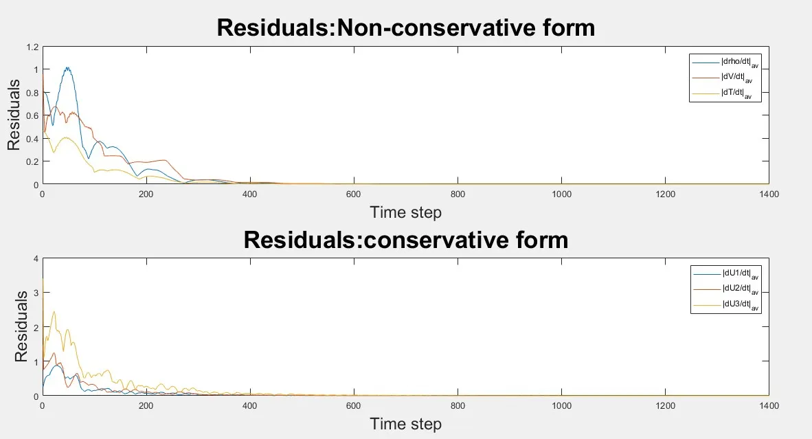
After time=600s solution reaching the steady-state. The residual plot of the flow variables is shown below. Conservative form with modified initial condition reaches steady-state faster than the non-conservative form.
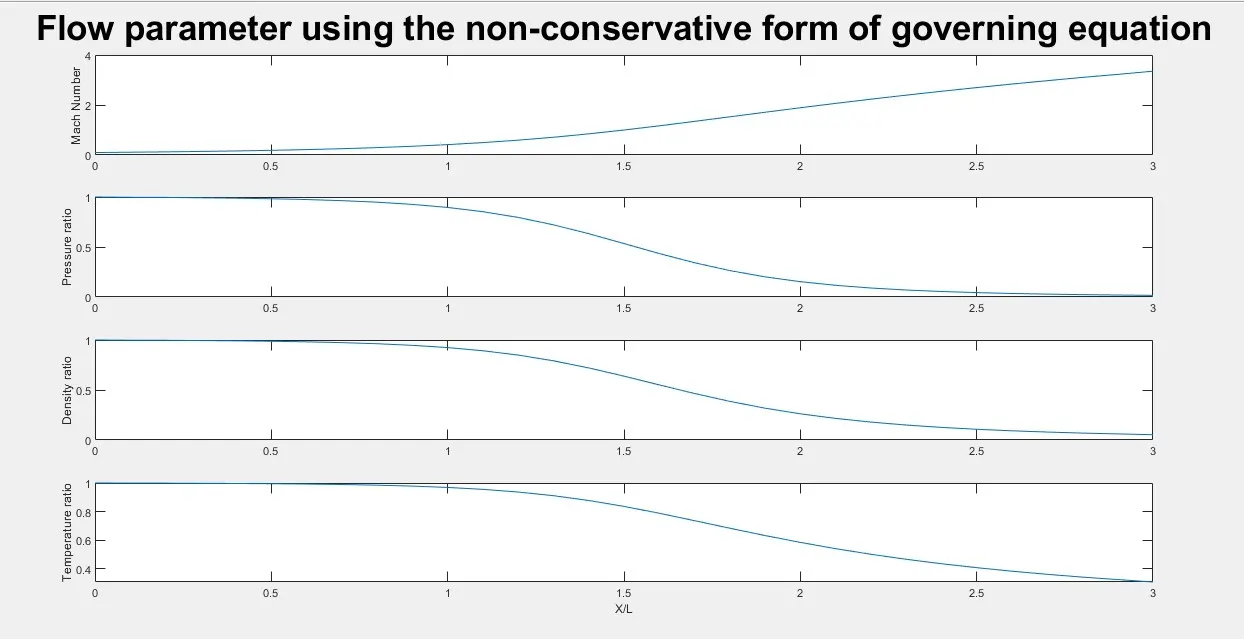
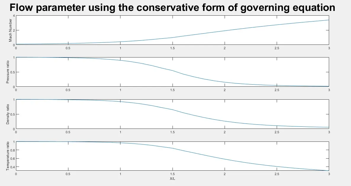
The steady-state flow variable along the length of the nozzle is obtained through a non-conservative and conservative form of the equations are shown below.
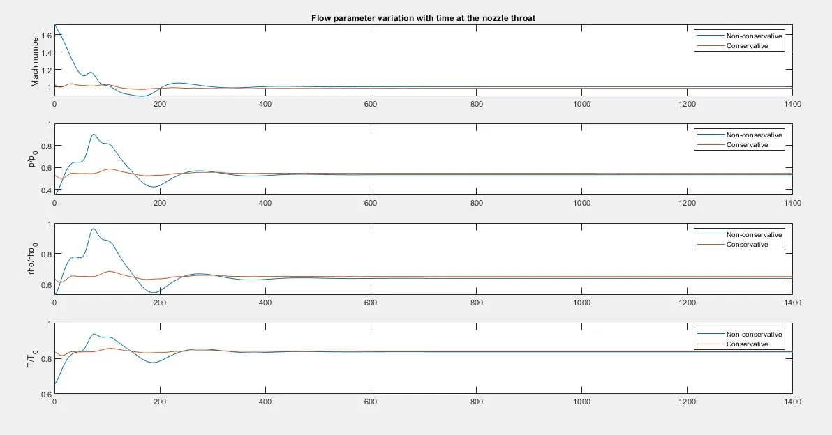
For the comparison, the flow variables at the throat section of the nozzle are plotted at each time step using a non-conservative and conservative form.
Variation of the mass flow rate along the length of the nozzle is shown below.
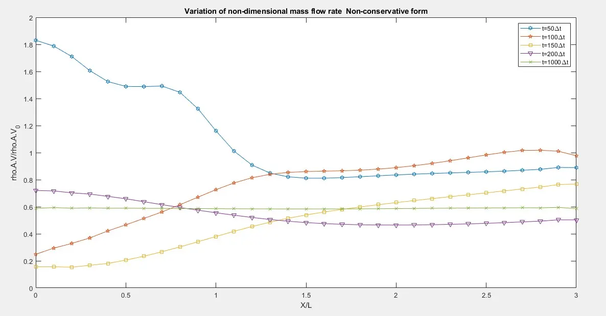
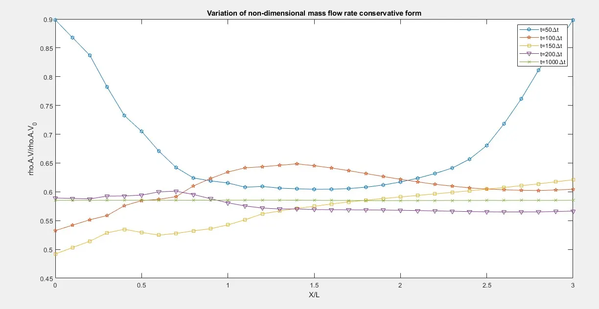
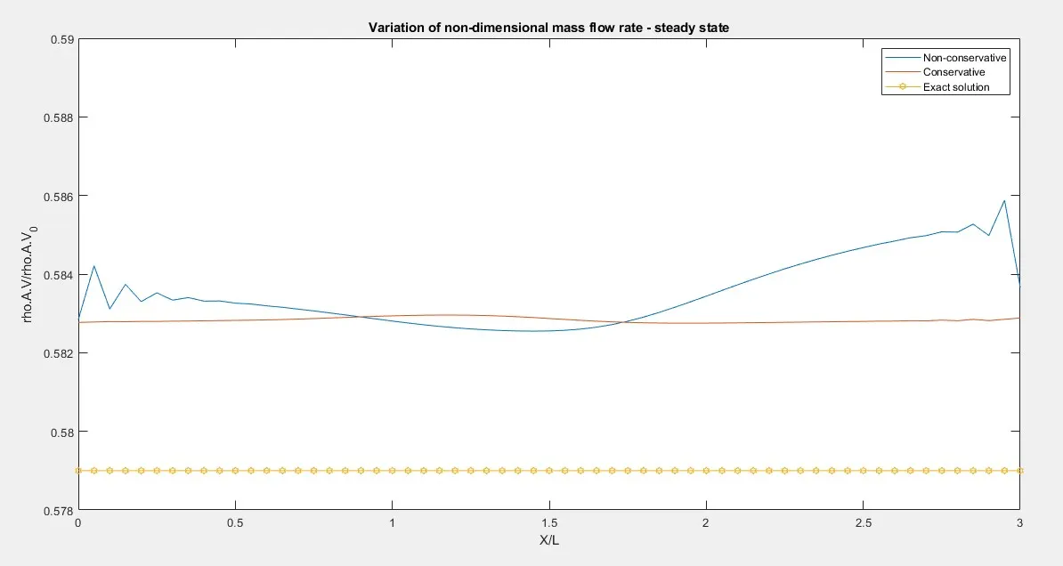
The mass flow rate along the length of the nozzle is compared with the exact value of the mass flow rate (0.579) at the end of the steady-state.
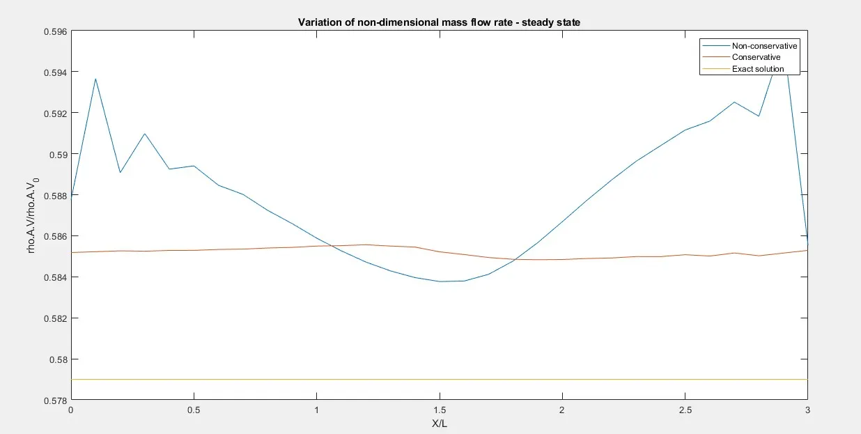
We can see that the conservative form gives almost constant mass flow but non-conservative has some fluctuation, it may be because of the extrapolation of the boundary condition.
For nx=51
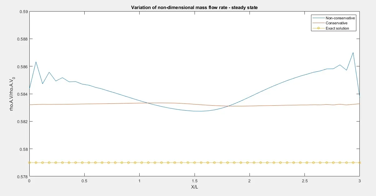
For the grid independency study, we compared the mass flow rate at the different numbers of the grid in increasing order, until we obtain minimum error between two cases.
For nx=61
For nx=71
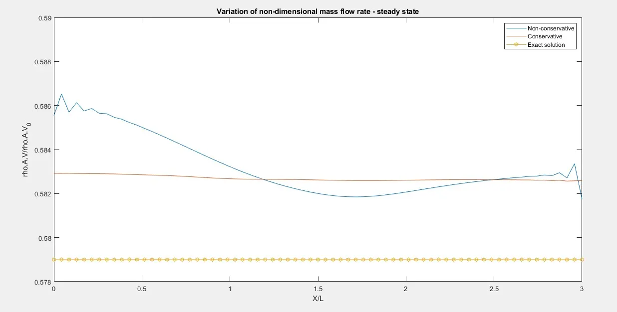
From the above figure, we can say that for any grid size conservative form is slightly effected whereas the non-conservative form shows huge variation. As the number of the grid increases conservative form reaches almost linear mass flow and the non-conservative form still struggling to reach the constant mass flow.
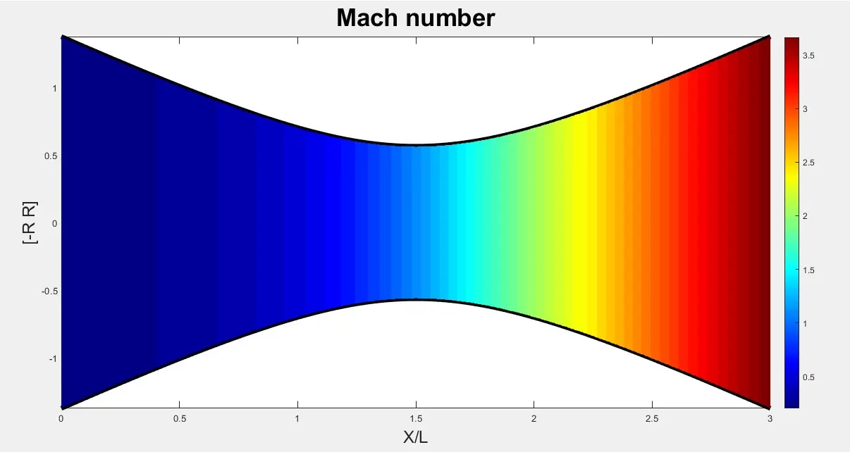
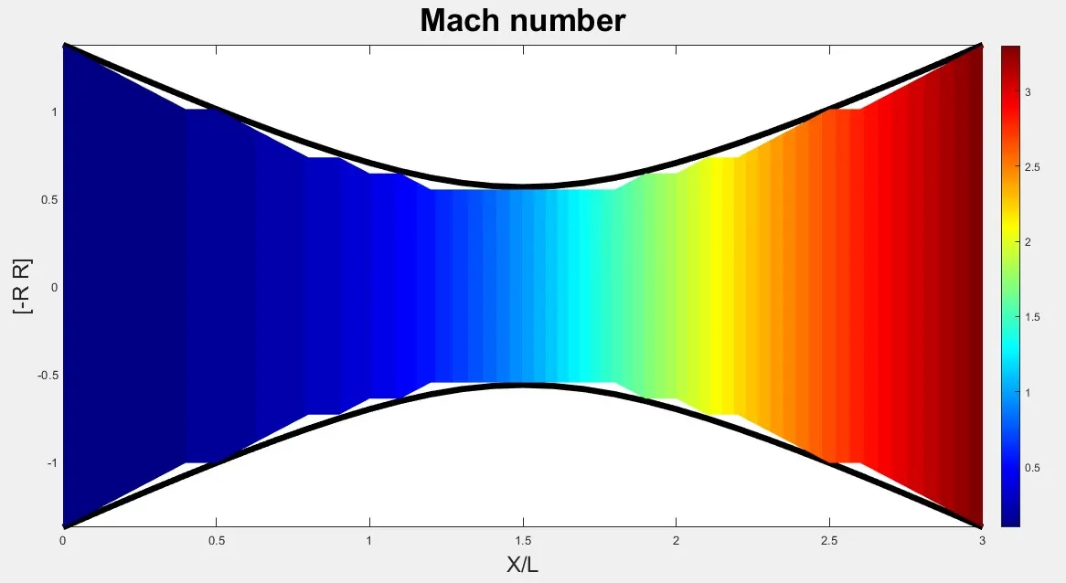
The Representation of the Mach number inside the nozzle geometry is shown below.
For nx=31
For nx= 601