Taylor table method and Matlab code

Aim: To derive the 4th order approximations of the second-order derivative.

Objective: To understand the different approximation schemes and write code to compare the scheme and analyze the plot.

Results:

The given function is f(x)=e^(x)*cos(x)=y

Second derivative of function is y’’= (-2*e^(x)*sin(x)).

1)Right skewed:

According to Taylor series forward skewed method

`Deltax^2*((d^2y)/(dx^2))` = a*f(i)+b*f(i+1)+c*f(i+2)+d*f(i+3)+e*f(i+4)+g*f(i+5)+higher_order_terms

By plotting Taylor table

	f(i)	Dx f’(i)	Dx f’’(i)	Dx f’’’(i)	Dx f1n(i)	Dx fn(i)
a*f(i)	a	0	0	0	0	0
b*f(i+1)	b	b	b/2	b/6	b/24	b/120
c*f(i+2)	c	2c	4c/2	8c/6	16c/24	32c/120
d*f(i+3)	d	3d	9d/2	27d/6	81d/24	243d//120
e*f(i+4)	e	4e	16e/2	64e/6	256e/24	1024e/120
g*f(i+5)	g	5g	25g/2	125g/6	625g/24	3125g/120
S=	0	0	1	0	0	0

By summing and valuating we get following algebraic equation:

a+b+c+d+e+g=0

0+b+2c+3d+4e+5g=0

0+b/2+ 4c/2+9d/2+16e/2+25g/2=1

0+ b/6+8c/6+27d/6+64e/6+125g/6=0

0+ b/24+16c/24+81d/24+256e/24+625g/24=0

0+ b/120+32c/120+243d//120+1024e/120+3125g/120=0

By converting coefficient into matrix form and by solving equation we get values for a,b,c,d,e,g.

Which gives,

a=15/4

b= (-77/4)

c=107/6

d= (-13)

e=61/12

g= (-5/6).

The higher_order_terms in the equation is of order 6 (o(Δx⁶)). While reducing the equation and by rearranging, the (o(Δx⁶)) reduces to (o(Δx⁴)). So the truncation error becomes 4^th order.

By substation, we get the equation as mentioned below. And it is the final equation used to solve the right-skewed scheme.

`(d^2y)/(dx^2)`=`((15/4)*f(i)+(-77/4)*f(i+1)+107/6*f(i+2)+(-13)*f(i+3)+61/12*f(i+4)+(-5/6)*f(i+5))/(Deltax^2)`

2) Left skewed:

The left-skewed scheme procedure is the same. But the equation differs.

`Deltax^2*((d^2y)/(dx^2))` = a*f(i)+b*f(i+1)+c*f(i+2)+d*f(i+3)+e*f(i+4)+g*f(i+5)+higher_order_terms

Taylor table will be as mentioned below:

	f(i)	Dx f’(i)	Dx f’’(i)	Dx f’’’(i)	Dx f1n(i)	Dx fn(i)
a*f(i)	a	0	0	0	0	0
b*f(i+1)	b	-b	b/2	-b/6	b/24	-b/120
c*f(i+2)	c	-2c	4c/2	-8c/6	16c/24	-32c/120
d*f(i+3)	d	-3d	9d/2	-27d/6	81d/24	-243d//120
e*f(i+4)	e	-4e	16e/2	-64e/6	256e/24	-1024e/120
g*f(i+5)	g	-5g	25g/2	-125g/6	625g/24	-3125g/120
S=	0	0	1	0	0	0

By substitution and solving algebraic equations final left-skewed equation as follows

`(d^2y)/(dx^2)`=`(15/4*f(i)+(-77/4)*f(i-1)+107/6*f(i-2)+(-13)*f(i-3)+61/12*f(i-4)+(-5/6)*f(i-5))/(Deltax^2)`

The higher_order_terms in the equation is of order 6 (o(Δx⁶)). While reducing the equation and by rearranging, the (o(Δx⁶)) reduces to (o(Δx⁴)). So the truncation error becomes 4^th order.

3) Central difference:

For the central difference scheme procedure is same. But equation differs,

`Deltax^2*((d^2y)/(dx^2))`= a*f(i-2)+b*f(i-1)+c*f(i)+d*f(i+1)+e*f(i+2)+higher_order_terms

Taylor table will be as mentioned below:

	f(i)	Dx f’(i)	Dx f’’(i)	Dx f’’’(i)	Dx f1n(i)	Dx fn(i)
a*f(i-2)	a	-2a	4a/2	-8a/2	16a/24	-32a/120
b*f(i-1)	b	-b	b/2	-b/6	b/24	-b/120
c*f(i)	c	0	0	0	0	0
d*f(i+1)	d	d	d/2	d/6	d/24	d//120
e*f(i+2)	e	2e	4e/2	8e/6	16e/24	32e/120
S=	0	0	1	0	0	?

By solving algebraic equations, we get,

a = (-1/12)

b = 4/3

c = (-5/2)

d = 4/3

e = (-1/12)

By the coefficient, the 5^th term will be zero and the higher_order_terms in the equation is of order 6 (o(Δx⁶)). While reducing the equation and by rearranging, the (o(Δx⁶)) reduces to (o(Δx⁴)). So, the truncation error becomes 4^th order.

By substitution and solving algebraic equations final central difference equation as follows,

`(d^2y)/(dx^2)`=`((-1/12)*f(i-2)+(4/3)*f(i-1)+(-5/2)*f(i)+(4/3)*f(i+1)+(-1/12)*f(i+2))/(Deltax^2)`

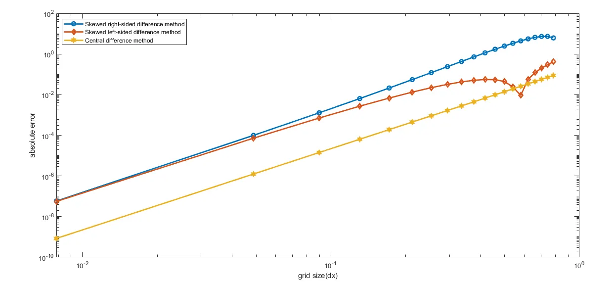
The absolute error of 3 approximations is shown above.

The central difference method gives the least error and the skewed right-side difference method gives a maximum error. An important point to be noted that after some point the absolute error starts to increase. In another way, this absolute error will decrease only until some range (only until finite grid size), further refinement in the grid will increase the error. The possible reason for this is numerical inaccuracy and truncation error.

clear all
close all
clc
%comparing the approximation methods for 4th order approximations of the second-order derivative. 
x=pi/3; %initial value
dx=linspace(pi/4,pi/400,20);
% dx = 1e-1:50:1e-4; %time range
%calculating analytical solution for second-order derivative of function f(x)=exp(x)*cos(x).
A_S=(-2*exp(x)*sin(x)) 
%looping to calculate the value of function in the range
for i=1:length(dx)
    a=dx(i); %assigning time step to a variable
   
%Skewed right-sided difference method calculation
    R_S(i)=(((15/4)*(exp(x)*cos(x))-(77/6)*(exp(x+a)*cos(x+a))+(107/6)*(exp(x+(2*a))*cos(x+(2*a)))-13*(exp(x+(3*a))*cos(x+(3*a)))+(61/12)*(exp(x+(4*a))*cos(x+(4*a)))-(5/6)*(exp(x+(5*a))*cos(x+(5*a))))/(a^2));
   
%Skewed left-sided difference method calculation
    L_S(i)=(((15/4)*(exp(x)*cos(x))-(77/6)*(exp(x-a)*cos(x-a))+(107/6)*(exp(x-(2*a))*cos(x-(2*a)))-13*(exp(x-(3*a))*cos(x-(3*a)))+(61/12)*(exp(x-(4*a))*cos(x-(4*a)))-(5/6)*(exp(x-(5*a))*cos(x-(5*a))))/(a^2));
    
%Central difference method calculation
    C_D(i)=(((-1/12)*(exp(x-(2*a))*cos(x-(2*a)))+(4/3)*(exp(x-a)*cos(x-a))-(5/2)*(exp(x)*cos(x))+(4/3)*(exp(x+a)*cos(x+a))-(1/12)*(exp(x+(2*a))*cos(x+(2*a))))/(a^2));
    
%Absolute error calculation
    E1(i)=abs(R_S(i)-A_S);
    
    E2(i)=abs(L_S(i)-A_S);
    
    E3(i)=abs(C_D(i)-A_S);
    
    
end
%plotting the graph
w=loglog(dx,E1,dx,E2,dx,E3);
 w(1).LineWidth = 2;
 w(2).LineWidth = 2;
 w(3).LineWidth = 2;
 w(1).Marker = 'o';
 w(2).Marker = 'd';
 w(3).Marker = 'h';
legend('Skewed right-sided difference method','Skewed left-sided difference method','Central difference method');
xlabel('grid size(dx)');
ylabel('absolute error');