Week 7 - Simulation of a 1D Super-sonic nozzle flow simulation using Macormack Method

MacCormack method

• In Computatonal flud dynamics ,the MacCormack method is popularly used discretization method for hyperbolic partial differential equation
• MacCormack method provides 2nd order accurate solution without the involvement of the 2nd derivative

Simulation of 1D supersonic nozzle flow:

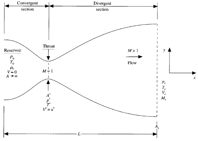
we discuss the physical properties of the flow through the convergent divergent nozzle.The convergent(subsonic) section connected with a reservior,so let us assume that inlet pressure,temperature and mach number as p0,T0,v0,&A=infinity,At subsonic the mach number is less than 1(M>1)

At throat area(sonic),A=A*,p=p*,t=t*&v*=a* mach number M=1.The sonic flow at the throat means that the local velocity at this location s equal to the local speed od sound and at divergence the flow expands to super sonic speed at the nozzle where the pressure,temperature,velocity and mach number are Pe,Te,Ve & Me.

The flow is locally subsonic in the convergen section of the nozzle,sonic at the throat and supersonic at the exit.The area of nozzle changes as the function of distance along the x axis.The flow field is two-dimensional(the flow varies in the two-dimesional xy space),we make assumption that the flow is only along x-axis.Such flow is defined as quasi-one-dimensional

MacCormack's Technique:

MacCormack's Techniques is the explicit finite difference technique which is second-order accurate in both space and time This method is very effective where we can obtain second-order accurate with first-order terms and mathematical complexity of calculating the second order time derivative can be avoided

In this method variable at the grid point (i,j) a time t+dt is calculated by using

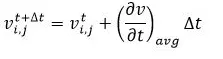
1.Intially,we start with initial conditions

With the help of intial conditions we calculate the predictor step

In this step,the spatial derivative on the right side are replaced with forward differences

consider Continuity equation

step1

step2

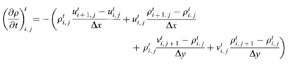
Predicted value of desity is calculated

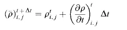
Corrector step:

Predicted value at time step (t+del(t)),(del(rho)/del(t))at t+del(t) is sub at corrector step

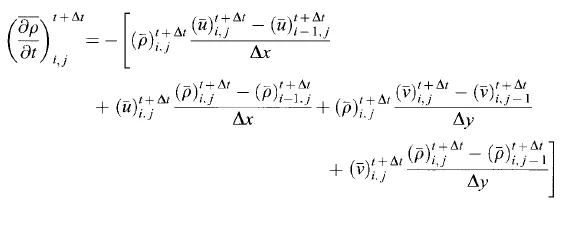
Then the average of corrector and predictor step are calculated

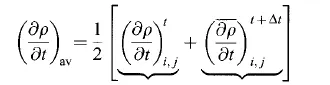
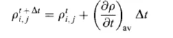
Once calculating the average value, the final solution is obtained

Governing equations for 1D Qausi supersonic nozzle flow

Governing equations are of two types

1.Conservative form

2.Non-Conservative form

Conservative form of equations

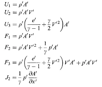
with the help of above elements,solution vector equations can be written as

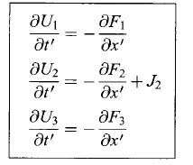
Once after solving the above equations our numerical solution vector U(U1,U2,U3) in steps of time,this the reason why U is called as Solution vector.In order to obtain primitive variables

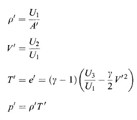
Boundary Conditions:

At inlet boundary Conditions the value U1 stays fixed and the other two solution vector U2 and U3 will float w.r.t time

U2=2*U2-U3;

U3=U1*((T/(gamma-1))+((gamma/2)*(v^2)))

At outlet boundary condition the values of solutionn vector of U1,U2 and U3 will change w.r.t time

U1(n)=(2*U1(n-1)-U1(n-2));

U2(n)=(2*U2(n-1))-U2(n-2);

U3(n)=(2*U3(n-1))-U3(n-2);

Intial conditions

Aera A=1+2.2*(x-1.5)^2 it remains constant throughout the nozzle

Velocity V=(0.59)/(rho*A);

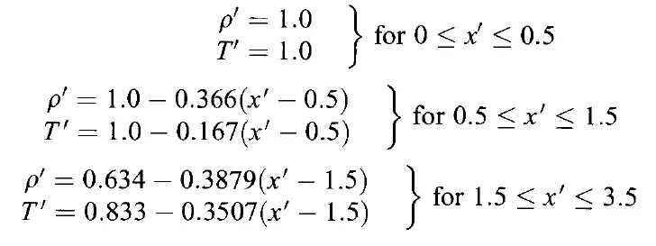
At t=0,values of density and temperature throughout the nozzle are given as follows

Non-Conservative form of equations:

Continuity

`(delrho)/(delt)=-rho*((delv)/(delx))-rho*V*((del(lanA))/(delx))-V*(delrho)/(delx)`

Momentum

`(delV)/(delt)=-V*(delV)/(delx)-(1/(gamma))*((delT)/(delx)+(T/rho))*(delrho)/(delx))`

Energy

`(delT)/(delt)=-V*(delT)/(delx)-(gamma-1)*T*((dv)/(dx)+(V)*(del(lanA/(delx))`

Calculation of time step

In this solution magnitude of time step is calculated based on the Courant number(C).The simple stablity analysis of linear hyperbolic eqations gives that any value of C less than 1 gives a satable solution

The magnitude of dt is calculated by using the formula

dt=C*(dx/(a+V));

With the help of the above formula,the value of dt is calculated at each every node Once after calculating the dt value at all the nodes minimum of all dt is considerd

Boundary conditions

At the inlet,the flow variables such as temperature and density remain constant and the value of velocity changes

V1=2*V2-V3;

At outlet conditions,all the flow variables keep on changing

V(n)=2*V(n-1)-V(n-2);

rho(n)=2*rho(n-1)-rho(n-2);

T(n)=2*T(n-1)-T(n-2);

Intial conditions

Aera A=1+2.2*(x-1.5)^2;

Density rho=1-(0.3146*x);

Temperature T=1-(0.2314*x);

Velocity V=(0.1+(1.09*x))*(T^0.5);

Conservative form

function[v,rho,t,m,mach,pr,v_t,rho_t,t_t,m_t,mach_t,pr_t]=non_conservative_form(n,L,c,nt,throat)

%input variables

x=linspace(0,L,n);
dx=x(2)-x(1);

rho=1-0.3146*x;
t=1-0.2314*x;
v=(0.1+1.09*x).*t.^0.5;
a=1+2.2*(x-1.5).^2;
gamma=1.4;
%calculating the value of time step based on courant number criteria
for i=1:n
    del_t(i)=c*(dx/(t(i)^0.5+v(i)));
end
dt=min(del_t);
%time loop
for k=1:nt
    rho_old=rho;
    v_old=v;
    t_old=t;
    %predictor method
for j=2:n-1
    dvdx=(v(j+1)-v(j))/dx;
    drhodx=(rho(j+1)-rho(j))/dx;
    dtdx=(t(j+1)-t(j))/dx;
    dlogadx=(log(a(j+1))-log(a(j)))/dx;
    % continuity equation
    drhodt_p(j)=-rho(j)*dvdx-rho(j)*v(j)*dlogadx-v(j)*drhodx;
    %momentum equation
    dvdt_p(j)=-v(j)*dvdx-(1/gamma)*(dtdx+(t(j)/rho(j))*drhodx);
    %energy equation
    dtdt_p(j)=-v(j)*dtdx-(gamma-1)*t(j)*(dvdx+v(j)*dlogadx);
    
    %solution update
    rho(j)=rho(j)+drhodt_p(j)*dt;
    v(j)=v(j)+dvdt_p(j)*dt;
    t(j)=t(j)+dtdt_p(j)*dt;
end
%corrector method
for j=2:n-1
    dvdx=(v(j)-v(j-1))/dx;
    drhodx=(rho(j)-rho(j-1))/dx;
    dtdx=(t(j)-t(j-1))/dx;
    dlogadx=(log(a(j))-log(a(j-1)))/dx;
    % continuity equation
    drhodt_c(j)=-rho(j)*dvdx-rho(j)*v(j)*dlogadx-v(j)*drhodx;
    %momentum equation
    dvdt_c(j)=-v(j)*dvdx-(1/gamma)*(dtdx+(t(j)/rho(j))*drhodx);
    %energy equation
    dtdt_c(j)=-v(j)*dtdx-(gamma-1)*t(j)*(dvdx+v(j)*dlogadx);
    
end
% average derivative
drhodt=0.5*(drhodt_p+drhodt_c);
dvdt=0.5*(dvdt_p+dvdt_c);
dtdt=0.5*(dtdt_p+dtdt_c);
%final solution update
for p=2:n-1
    rho(p)=rho_old(p)+drhodt(p)*dt;
    v(p)=v_old(p)+dvdt(p)*dt;
    t(p)=t_old(p)+dtdt(p)*dt;
    
end
%inlet
v(1)=2*v(2)-v(3);
%outlet
v(n)=2*v(n-1)-v(n-2);
rho(n)=2*rho(n-1)-rho(n-2);
t(n)=2*t(n-1)-t(n-2);
% calculating solution
m=rho.*v.*a;
mach=v./((t).^0.5);
pr=rho.*t;
%throat values
rho_t(k)=rho(throat);
t_t(k)=t(throat);
pr_t(k)=pr(throat);
mach_t(k)=mach(throat);
v_t(k)=v(throat);
m_t(k)=m(throat);

figure(1)
    if k==50
        plot(x,m,'b','linewidth',2);
        hold on
    elseif k==100
        plot(x,m,'g','linewidth',2);
        hold on
    elseif k==150
        plot(x,m,'c','linewidth',2);
        hold on
    elseif k==200
        plot(x,m,'y','linewidth',2);
        hold on
    elseif k==550
        plot(x,m,'b','linewidth',2);
    elseif k==700
        plot(x,m,'r','linewidth',2);
    elseif k==1400
        plot(x,m,'m','linewidth',2);
       
        grid on
        ylabel('Non-dimesional mass flow rate','fontweight','bold','fontsize',11);
        xlabel('Non-Dimensional dstance through nozzle(x)','fontsize',12,'fontweight','bold');
        title('Non_dimesional mass flow rate(Non-Conservative form) along x,at different time steps','Fontsize',12,'fontweight','bold','color','r');
        legend({'50 time step','100 time step','150 time steps','200 time steps','550 time steps','700 time steps','1400 time steps'});
        
        
    end
end

end

Non-Conservative Form

function[v,rho,t,m,mach,pr,v_t,rho_t,t_t,m_t,mach_t,pr_t]=non_conservative_form(n,L,c,nt,throat)

%input variables

x=linspace(0,L,n);
dx=x(2)-x(1);

rho=1-0.3146*x;
t=1-0.2314*x;
v=(0.1+1.09*x).*t.^0.5;
a=1+2.2*(x-1.5).^2;
gamma=1.4;
%calculating the value of time step based on courant number criteria
for i=1:n
    del_t(i)=c*(dx/(t(i)^0.5+v(i)));
end
dt=min(del_t);
%time loop
for k=1:nt
    rho_old=rho;
    v_old=v;
    t_old=t;
    %predictor method
for j=2:n-1
    dvdx=(v(j+1)-v(j))/dx;
    drhodx=(rho(j+1)-rho(j))/dx;
    dtdx=(t(j+1)-t(j))/dx;
    dlogadx=(log(a(j+1))-log(a(j)))/dx;
    % continuity equation
    drhodt_p(j)=-rho(j)*dvdx-rho(j)*v(j)*dlogadx-v(j)*drhodx;
    %momentum equation
    dvdt_p(j)=-v(j)*dvdx-(1/gamma)*(dtdx+(t(j)/rho(j))*drhodx);
    %energy equation
    dtdt_p(j)=-v(j)*dtdx-(gamma-1)*t(j)*(dvdx+v(j)*dlogadx);
    
    %solution
    rho(j)=rho(j)+drhodt_p(j)*dt;
    v(j)=v(j)+dvdt_p(j)*dt;
    t(j)=t(j)+dtdt_p(j)*dt;
end
%corrector method
for j=2:n-1
    dvdx=(v(j)-v(j-1))/dx;
    drhodx=(rho(j)-rho(j-1))/dx;
    dtdx=(t(j)-t(j-1))/dx;
    dlogadx=(log(a(j))-log(a(j-1)))/dx;
    % continuity equation
    drhodt_c(j)=-rho(j)*dvdx-rho(j)*v(j)*dlogadx-v(j)*drhodx;
    %momentum equation
    dvdt_c(j)=-v(j)*dvdx-(1/gamma)*(dtdx+(t(j)/rho(j))*drhodx);
    %energy equation
    dtdt_c(j)=-v(j)*dtdx-(gamma-1)*t(j)*(dvdx+v(j)*dlogadx);
    
end
% average derivative
drhodt=0.5*(drhodt_p+drhodt_c);
dvdt=0.5*(dvdt_p+dvdt_c);
dtdt=0.5*(dtdt_p+dtdt_c);
%final solution update
for p=2:n-1
    rho(p)=rho_old(p)+drhodt(p)*dt;
    v(p)=v_old(p)+dvdt(p)*dt;
    t(p)=t_old(p)+dtdt(p)*dt;
    
end
%inlet
v(1)=2*v(2)-v(3);
%outlet
v(n)=2*v(n-1)-v(n-2);
rho(n)=2*rho(n-1)-rho(n-2);
t(n)=2*t(n-1)-t(n-2);
% calculating solution
m=rho.*v.*a;
mach=v./((t).^0.5);
pr=rho.*t;
%throat values
rho_t(k)=rho(throat);
t_t(k)=t(throat);
pr_t(k)=pr(throat);
mach_t(k)=mach(throat);
v_t(k)=v(throat);
m_t(k)=m(throat);

figure(1)
    if k==50
        plot(x,m,'b','linewidth',2);
        hold on
    elseif k==100
        plot(x,m,'g','linewidth',2);
        hold on
    elseif k==150
        plot(x,m,'c','linewidth',2);
        hold on
    elseif k==200
        plot(x,m,'y','linewidth',2);
        hold on
    elseif k==550
        plot(x,m,'b','linewidth',2);
    elseif k==700
        plot(x,m,'r','linewidth',2);
    elseif k==1400
        plot(x,m,'m','linewidth',2);
       
        grid on
        ylabel('Non-dimesional mass flow rate','fontweight','bold','fontsize',11);
        xlabel('Non-Dimensional dstance through nozzle(x)','fontsize',12,'fontweight','bold');
        title('Non_dimesional mass flow rate(Non-Conservative form) along x,at different time steps','Fontsize',12,'fontweight','bold','color','r');
        legend({'50 time step','100 time step','150 time steps','200 time steps','550 time steps','700 time steps','1400 time steps'});
        
        
    end
end

end

Main Program

clear all
close all
clc

%input
n=31;
L=3;
x=linspace(0,L,n);
dx=x(2)-x(1);
c=0.5;
throat=((n-1)/2)+1;
gamma=1.4;
nt=1400;
%
tic;
[v,rho,t,m,mach,pr,v_t,rho_t,t_t,m_t,mach_t,pr_t]=non_conservative_form(n,L,c,nt,throat);
Non_conservative_simulation_time=toc

tic;
[v2,rho2,t2,m2,mach2,pr2,v_t2,rho_t2,t_t2,m_t2,mach_t2,pr_t2]=conservative_form(n,L,c,nt,throat)
Conservative_exection_time=toc;

%varaition of flow parameters at the throat
figure(3)
a1=subplot(4,1,1);
plot(linspace(1,nt,nt),rho_t,'b');
hold on
plot(linspace(1,nt,nt),rho_t2,'color','r');
grid on;
ylabel('rho','fontsize',12,'fontweight','bold');
title('Timewise varition of flow parameters at throat','fontsize',12,'color','r','fontweight','bold');
h=legend('Non-conservative form','Conservative Form');
set(h,'Location','northeastoutside')


a2=subplot(4,1,2);
plot(linspace(1,nt,nt),t_t,'b');
hold on
plot(linspace(1,nt,nt),t_t2,'color','r');


grid on;
ylabel('T','Fontsize',12,'fontweight','bold');
h=legend('Non-conservative form','Conservative Form');
set(h,'Location','northeastoutside')

a3=subplot(4,1,3);
plot(linspace(1,nt,nt),pr_t,'b');
hold on
plot(linspace(1,nt,nt),pr_t2,'color','r');
grid on;
ylabel('Pr','Fontsize',12,'fontweight','bold');
h=legend('Non-conservative form','Conservative Form');
set(h,'Location','northeastoutside')

a4=subplot(4,1,4);
plot(linspace(1,nt,nt),mach_t,'b');
hold on
plot(linspace(1,nt,nt),mach_t2,'color','r');
grid on;
ylabel('Ma','Fontsize',12,'fontweight','bold');
xlabel('No of time step','fontweight','bold');
h=legend('Non-conservative form','Conservative Form');
set(h,'Location','northeastoutside')




%Variatiation in flow parameters along x axis
figure(4)
p1=subplot(4,1,1);
plot(x,mach,'b');
hold on
plot(x,mach2,'r*','markersize',3);
grid on;
ylabel('Ma','fontsize',12,'fontweight','bold');
hold on
h=legend('Non-conservative form','Conservative Form');
set(h,'Location','northeastoutside')
title('varition of flow parameters along x-axis','fontsize',12,'color','r','fontweight','bold')



p2=subplot(4,1,2)
plot(x,pr,'b');
hold on
plot(x,pr2,'r*','markersize',3);
grid on;
ylabel('Pr','fontsize',12,'fontweight','bold');
h=legend('Non-conservative form','Conservative Form');
set(h,'Location','northeastoutside')


p3=subplot(4,1,3)
plot(x,rho,'b');
hold on
plot(x,rho2,'r*','markersize',3);
grid on;
ylabel('rho','fontsize',12,'fontweight','bold');
h=legend(p3,{'Non-Conservative Form','Coservative Foam'});
set(h,'location','northeastoutside')

p4=subplot(4,1,4)
plot(x,t,'b');
hold on
plot(x,t2,'r*','markersize',3);
grid on;

h=legend(p4,{'Non-Conservative Form','Coservative Foam'});
set(h,'location','northeastoutside')

ylabel('T','fontsize',12,'fontweight','bold');
xlabel('Non-Dimensional length','fontweight','bold');

%mass flow rate comparision between two forms of equation
figure(5)


plot(x,m,'r','linewidth',1.5)
hold on
plot(x,m2,'b','linewidth',1.5)
hold on

ylabel('Non-dimensional mass flow rate','fontsize',12,'fontweight','bold');
xlabel('Non-dimensional distance through nozzle(x)','fontsize',12,'fontweight','bold');
h=legend('Non-conservative form','Conservative Form');
set(h,'Location','northwest')
title('Non-dimensional mass flow rate comparison','fontweight','bold','fontsize',12,'color','r');
axis([0 3 0.575 0.600]);
grid on

Steady-state distribution of primitive variables inside the nozzle

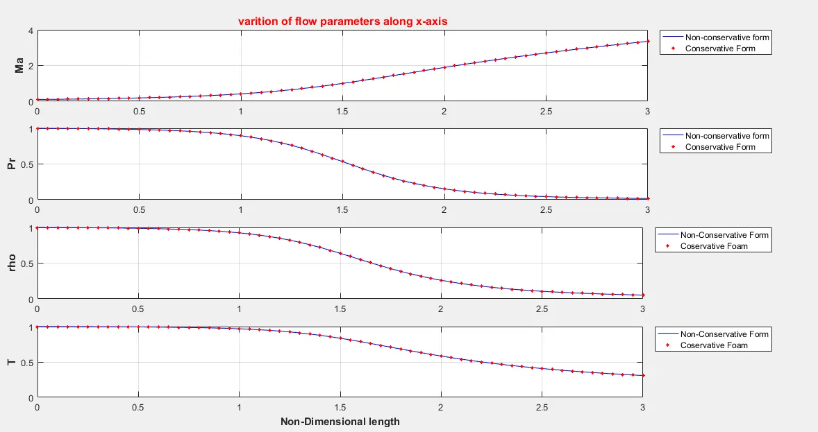
1Both forms produce almost similar plots ,once after the attainment of a steady state at 1400 time step are carried out by the time marching approach,at which the steady state is almost obtained where it is equal to exact analytical solution

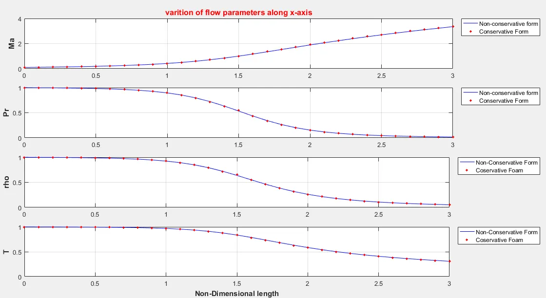
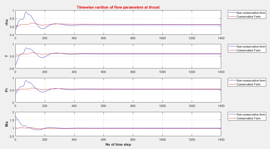
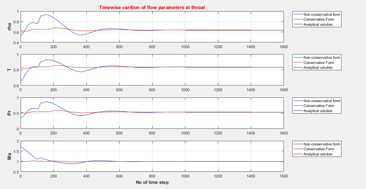
2.Time varition of flow parameter along the non-dimensional lenght of nozzle at throat

• From the below graphs we found that the solution of Non-Conservative form lies closer to exact values of rho,T,pr and mach When compared to the conservative form soution
• The above values of flow parameter at a particular region is a good way of investigating the attainment of steady-state by the system
• The non-consevative form generate more accurate results for primitive varibles
• But even after 1400 time steps,residue(Difference between the numerical solution and exact solution)exists,for a non-conservative form,the value of residue will be almost constant after 1400 time step equal,for a conservative form the value of residue will be almost constant after 1400 time step and is equal to 10^-3
• Non-conservative form leads to smaller residue,and the quality index is determined by the rate of decay of the residue
• From the plots below it can be seen thatthe steady-state is almost obtained with agood level of approximation,after 500 time steps for pratical purposes.But this evidence is not evidence is not enough to justify our observation

NON-CONSERVATIVE FORM

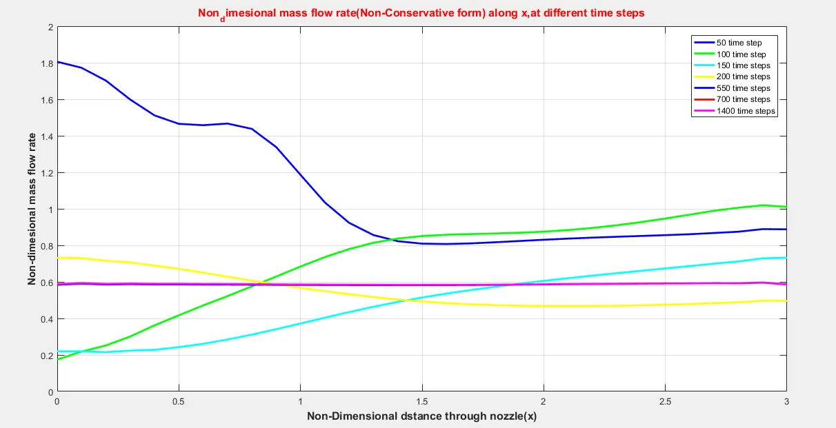
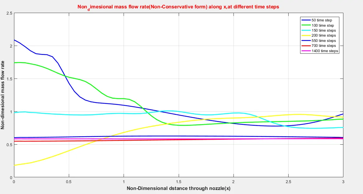
Non-Dimensional Mass Flow rate behaviour Along Non-Dimensional lenght of nozzle

• From the above figure it shows that the mass flow rate curve obtained for 1400 time steps are almost overlaying in the same region of space
• so this plot substance our previous assumption from the observation of the ''Timewise varition of flow parameters at the nozzle throat",after 500 time step almost steady state is obtained for the non-conservative form the flow equation
• but in theoretically it take infinity time step to obtain a steady-state

2.Conservative Form

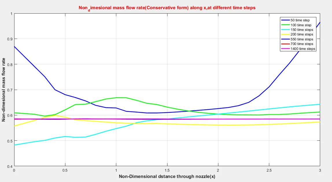
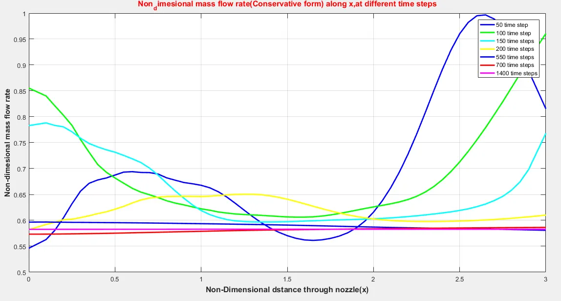
1.when compared to the previous plot, the fluctuation are less severe in the conservative form.But comparing these two plots makes no sense because we assumed different sets of intial conditions.In fact,we mad ean intelligent guess while choosing the intial conditions(density,temperature,velocity)with he constant mass flow for the conservative form because of the sensitiviy behavior.This is the reason for its mild fluctuating behaviour.

2. Even from this plot,it can be observed that the mass flow rate curve obtained for 550,700 and 1400 steps are almost overlying in the same region of space.

3.But,the reasonable settlement of the fluctuations at 550th time step may be due to the more realistic initial conditions with constant mass flow,assumed by the intelligent guess.And also for conservative form,the value of residue at 550th time step will be somewhere between 10^-1(intially)and 10^-3(after 1400 timesteps),which doesn't leads to a good approximation with exact solution@ 550th time step milder fluctuation still exist,which can't be approximated with the exat solution at a good level of accuracy,due to the presence of large values of residue

4.After 700 time steps,it almost(but not quite) becomes equal to a constant value.Moreover,it is quite close to exact analytical solution of 0.579 and therefore the steady state is almost obtained (for practical purposes).Theoretically,it takes infinite time steps to attain a steady state

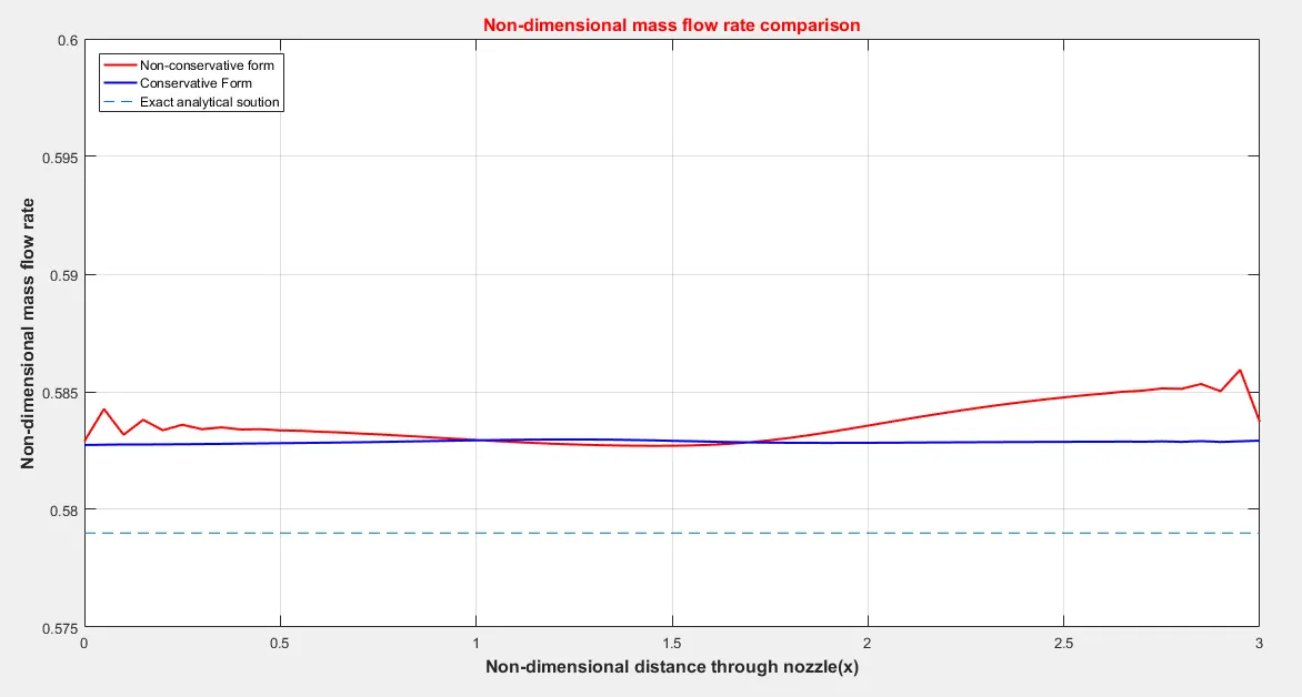
Comparison of steady stae mass flow plots of two different forms of the equation

1.The conservative form generates abetter mass flow distribution with fewer fluctuations when compared with non-conservative form

2.The reason is the mass flow itself is one of the dependent variables in the equations of the conservative form,whereas in the non-conservative form,the dependent variables are the primitive variables and the mass flow is obtained after some calculation

3.Conservative form generates more accurate results for the flux varibles.

what are the factors which influence the residue ?how to reduce the value of residue?

1 Small inflow boundary condition error:

we assumed tht the density,temperature and pressure at the inlet are equal to the reservior properties.This is only true if Mach number at inlet is equal to zero.But Mach number is a function of area ratio A/A*.Even at the inlet finite value exists for the area ratio(5.95),and hence there must be a finite Mach number at the inlet (x=0),both numerically and analytically .It is not viewed as serious

2.Courant number effects

According to the Courant number stability criteria,the CFL number must be less than or equal to 1.But we assumed C=0.5 which is smaller than necessary at which the solution is stable and the results are closer to exact analytical soution(calculations are not presented,as it is out of the scope of this project).So,we can conclude that we made a safe guess.CFL criteria provide a good esitimate to calculate the time step value for even nonlinear hyperbolic partial differential equation(Quasi 1D nozzle flow),but it does not hold exactly because it is derived for linear hyperbolic equations.

3.Grid dependence

1.Even if the nuber of grid points is doubled,and there is only a marginal difference in the solution ,then our orginal calculation with the intial no of grid points are said to be GRID INDEPENDENT

2.This factor is purely based on circumstances,by depending upon the expected order of accuracy and the allowable range of tolerance

3.In our case we assumed n=31,so let's check whether it is grid-independent or not.Intiallly,to start the discussion it would be better if we plot the graphs with respect to the modified value of n i.e,n=61.When modifying the value of 'n',the number of time steps should also be modified,so that the elapsed non-dimensional time is same for both cases.By doing so,the grid independence test can be carried out by comparing the curves obtained for both caese,at a particular non-dimensional time.

4.The total non-dimensional time elapsed(n=31),is equal to dt*no of time steps Initially dt is calculated to all the grid points from i=1 to n using the CFL criteria,and then the smallest of all the values is chosen as 'dt'.By following this approach the same value of dt will be used throughoutthe time marching.So that there wont be artificial time wrap and it provides a time accurate solution of actual transient flow field

5 the value of non-dimensional time elapsed (n=31) is 0.02036 for non-conservative and conservative forms repectively.let's choose the higher value for consideration.Therefoere the total non-dimensional time elapsed,0.02036*1400=28.50

6.The value of non-dimensional time step(n=61) is found similarly and it is equal to 0.010181.So,the simulation should run for higher no of time steps to reach the non-dimensional time of magnitude 28.50.The reason why it takes higher no of time steps is because the no time step reduces as the no of grid points are increased

7.No of time steps required for n=61 is (28.50/0.010181)=2800 time steps approximately it seems to be almost double in our case ,i.e in other words ,for n=31 the curves produced at 100th time step ,500th time stepand 1400 time step will be similar,to the curves generated for n=61 at 200th time step ,1000th time step and 2800th time step respectively if our intial assumption n=31 is grid independent

8.Grid independence test can be also carrived out by comparing the value obtained by conservative and non-conservative forms at the throat, for n=31 and 61.It has to be noted that the non-conservative forms at the throat for n=31 and 61.It has to be noted that the non-conservative form results are more accurate when compared with the conservative form results. Even though by doubling the number of grid points,th solution of the conservative form with half as many grid points i.e,n=31.Therefore for pratical purposes,n=31 can be treated as grid-independent.

First,let's observe the below plots for n=61,and compare it with the plots generated for n=31.As expected,the plots obtained for n=31 and 61 seem to possess similar curves at the same elapsed non-dimensional time.Minor variationof values are observed,but for practical purposes,n=31 can be treated as grid-independent.

Qualitative aspects of quasi 1D nozzle flow:isentropic subsonic-supersonic solution(n=61)

Timewise variation of flow parameters at the nozzle throat (n=61)

Non-dimensional Mass flow rate behavior along the non-dimensional length of nozzle

A.Non-Conservative Form

1.for n=61,almost steady state is obtained after 1000 time steps(can be observed from the below graph),i.e at the non-dimensional time (0.010181*1000)=10.81,which is equal to(10.181/0.0236)=500 time steps for n=31

2 This way of checking even provides better evidence for the grid-independence nature for n=31 for practical purposes

Conservative Form

Comparision of steady state mass flow plots of two different forms of the equation

Which method is faster ?

For n=61,c=0.5

Non_conservative_simulation_time=56.883

Conservative_simulation_time=59.244

For n=31,c=0.5

Non_conservative_simulation_time =15.943

Conservative_simulation_time=16.440

In the case of conservative form,primitive variables need to be decoded from the flux variables, but this is not necessary in case of non-conservativeform.And therefore solving form requires more computational time