Challenge

Week 7 - Simulation of a 1D Super-sonic nozzle flow simulation using Macormack Method

AAshish Sharma25 Oct 2022

Aim - Simulation of 1D SuperSonic Nozzle flow.

Objective -

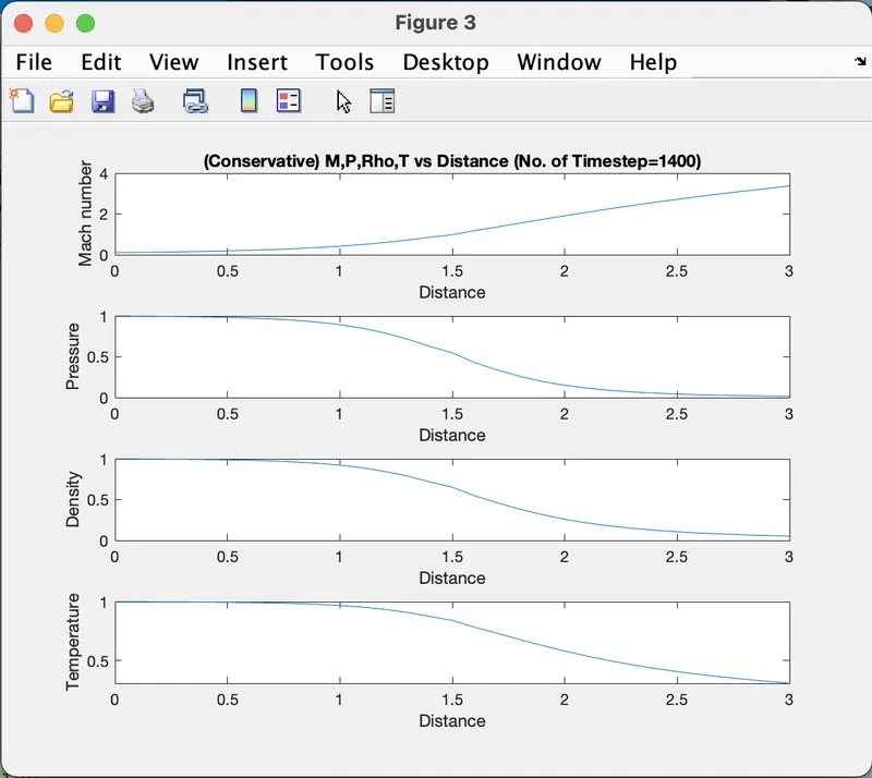
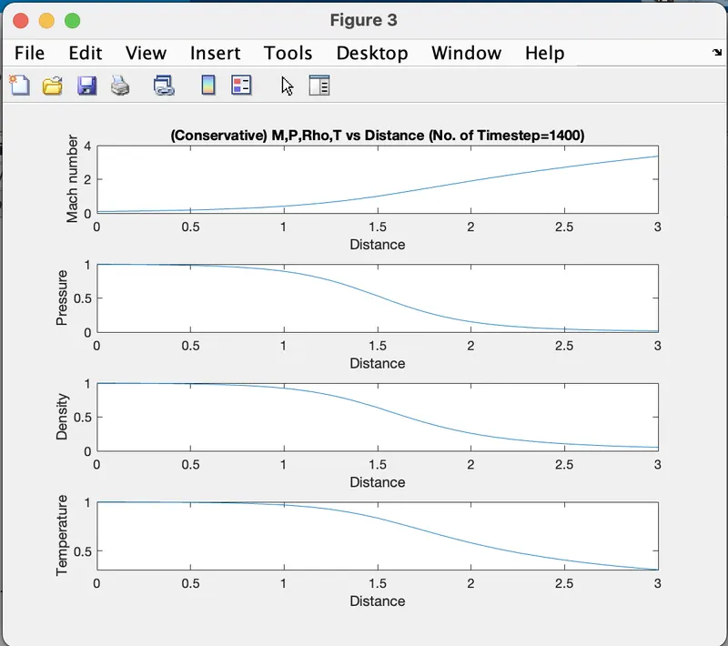
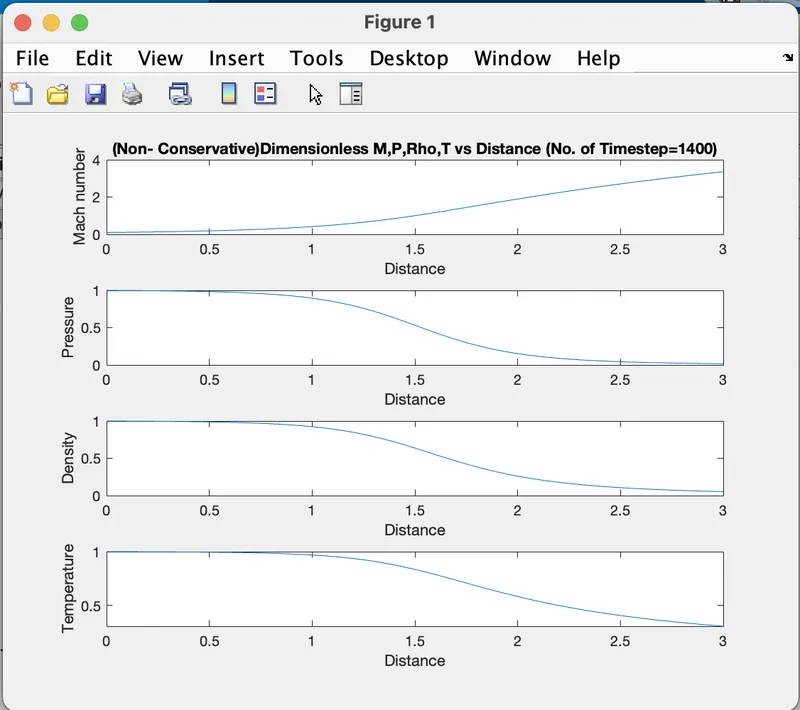
Steady-state distribution of primitive variables inside the nozzle.
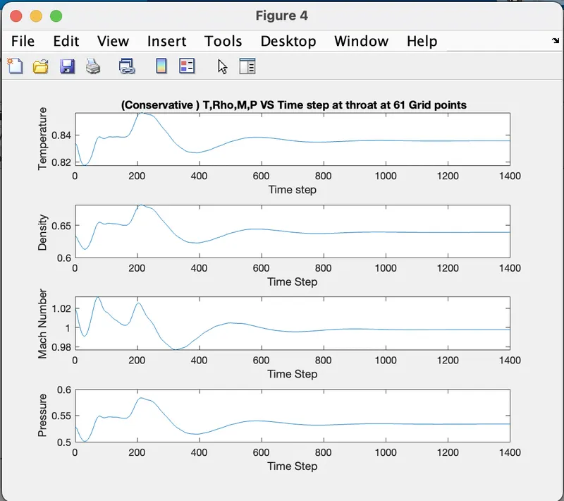
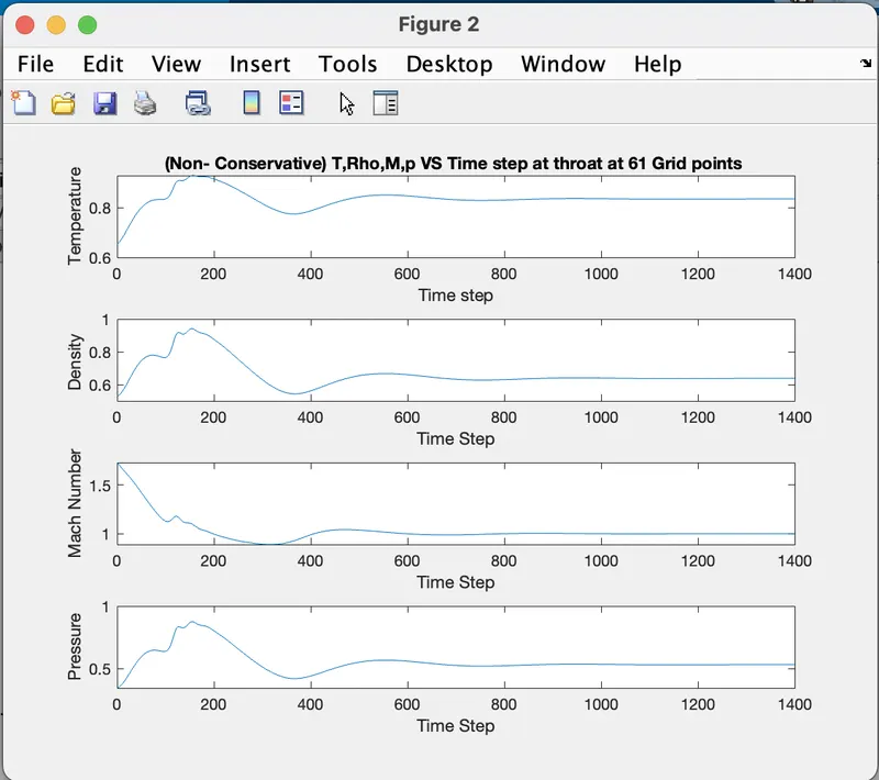
Time-wise variation of the primitive variables.
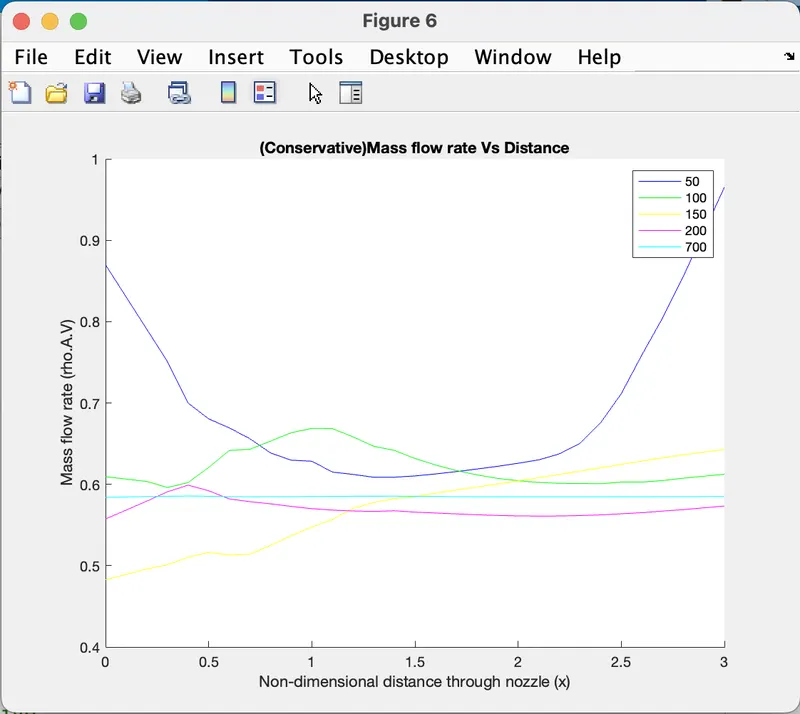
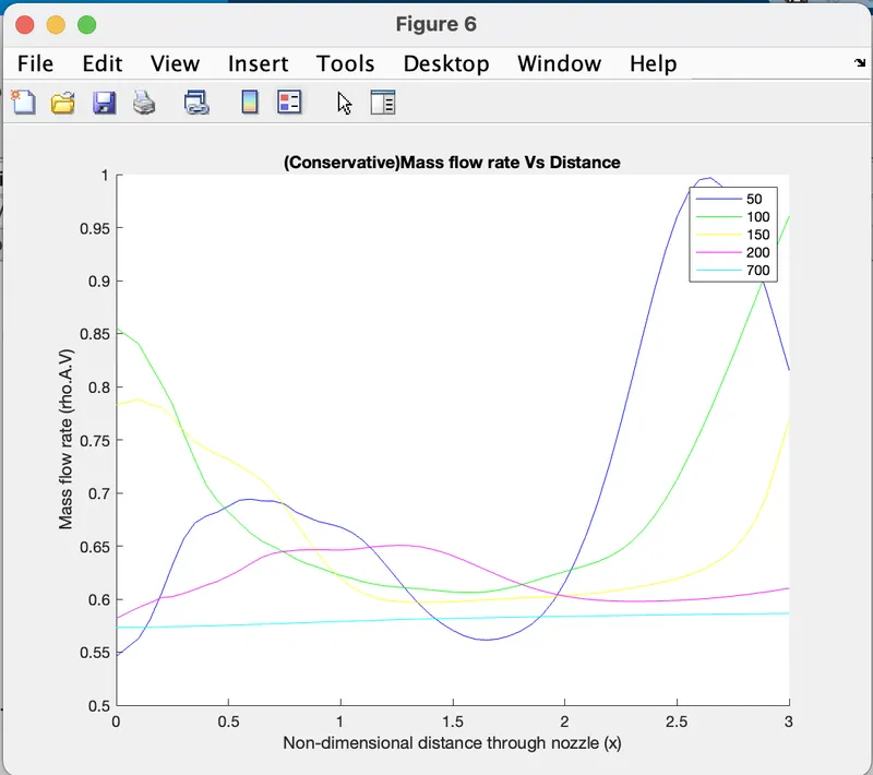
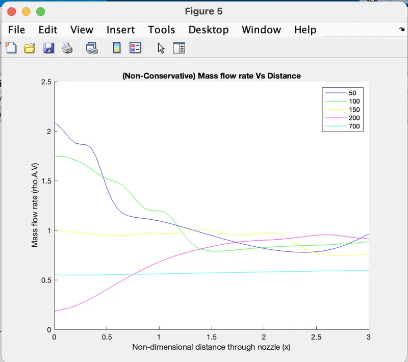
Variation of Mass flow rate distribution inside the nozzle at different time steps during the time-marching process.
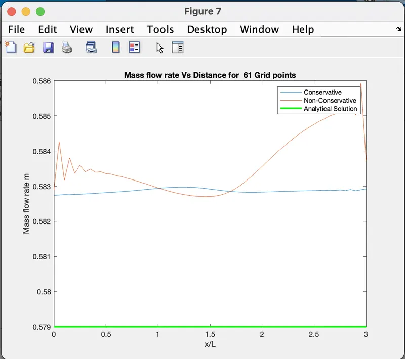
Comparison of Normalized mass flow rate distributions of both forms.

Theory -

Any numerical solution of isentropic flow though a quasi 1D subsonic-supersonic nozzle is unreasonable, while analytic solution exists for these kind of problems. However we are trying here to establish the broadened capability of CFD in various streams rather in representing the approximated form of anayltic solution. Here, we implement the numerical solution with Conservative and Non-Conservative forms.

Governing Equations are marched in terms of PDE for both forms in order to use Time Marching solution for the problem. These forms represent in numerical aspect only, if we analytic all the methods are same.

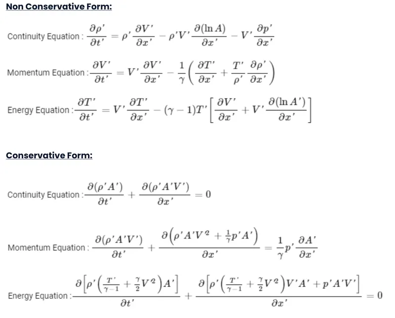
Given below are the governing equations for quasi-one -dimesional flow -

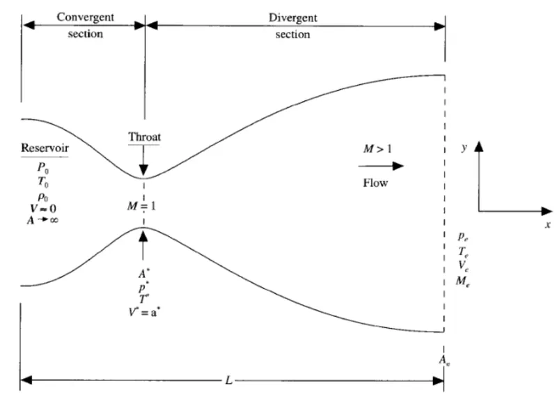
Nozzle diagram -

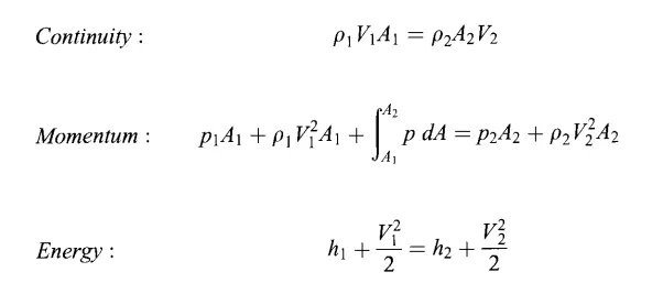
MacCarmack method -

To discretize the numerical solution we use the technique called MacCarmack method. The MacCormack method is a variation of the two-step Lax-Wendroff Scheme but is much simpler in application.

The application of MacCormack method proceeds in two steps; a predictor step which is followed by a corrector step.

Program Code -

% 1D SuperSonic flow through a convergent-divergent nozzle.

clear
close
clc

n=input('Enter number of grid points ');
x=linspace(0,3,n);
gamma=1.4;
dx=x(2)-x(1);


%area
 a=1+(2.2*(x-1.5).^2);

% timestep
nt=1400;

% Non -conservative 
[rho,v,t,M,p,m,p_t,rho_t,t_t,M_t]=non_conservative(n,nt);

%Conservative
[rho_c,v_c,t_c,M_c,p_c,m_c,p_tc,rho_tc,t_tc,M_tc]= conservative(n,nt);


% Non -conservative

% To plot variables Vs distance
figure(1)
subplot (4,1,1)
plot(x,M)
title_text=sprintf('(Non- Conservative)Dimensionless M,P,Rho,T vs Distance (No. of Timestep=%d)',nt);
title(title_text)
xlabel('Distance')
ylabel('Mach number')
hold on

subplot(4,1,2)
plot(x,p)
xlabel('Distance')
ylabel('Pressure')
hold on
   
subplot(4,1,3)
plot(x,rho)
xlabel('Distance')
ylabel('Density')
hold on

subplot(4,1,4)
plot(x,t)
xlabel('Distance')
ylabel('Temperature')
hold on

% To plot variables at time step 
figure(2)
nt=1:1400 ;
subplot(4,1,1)
plot (nt,t_t)
 title_text=sprintf( '(Non- Conservative) T,Rho,M,p VS Time step at throat at %d Grid points ',n);
 title(title_text)
xlabel('Time step')
ylabel('Temperature')
hold on

subplot(4,1,2)
plot(nt,rho_t)
xlabel('Time Step')
ylabel('Density ')
hold on

subplot(4,1,3)
plot(nt,M_t)
xlabel('Time Step')
ylabel('Mach Number')
hold on

subplot(4,1,4)
plot(nt,p_t)
xlabel('Time Step')
ylabel('Pressure')
hold on

% Conservative 
nt=1400 ;
figure(3)
subplot(4,1,1)
plot(x,M_c)
title_text=sprintf('(Conservative) M,P,Rho,T vs Distance (No. of Timestep=%d)',nt);
title(title_text)
xlabel('Distance')
ylabel('Mach number')
hold on

subplot(4,1,2)   
plot(x,p_c)

xlabel('Distance')
ylabel('Pressure')
hold on

subplot(4,1,3)
plot(x,rho_c)
xlabel('Distance')
ylabel('Density')
hold on

subplot(4,1,4)
plot(x,t_c)


xlabel('Distance')
ylabel('Temperature')
hold on

figure(4)
nt=1:1400 ;
subplot(4,1,1)
plot (nt,t_tc)
title_text=sprintf( ' (Conservative ) T,Rho,M,P VS Time step at throat at %d Grid points',n);
title(title_text)
xlabel('Time step')
ylabel('Temperature')
hold on

subplot(4,1,2)
plot(nt,rho_tc)

xlabel('Time Step')
ylabel('Density ')
hold on

subplot(4,1,3)
plot(nt,M_tc)

xlabel('Time Step')
ylabel('Mach Number')
hold on

subplot(4,1,4)
plot(nt,p_tc)

xlabel('Time Step');
ylabel('Pressure');
hold on


figure(7)
plot(x,m_c)
hold on
plot(x,m)
line([0 3],[0.579 0.579],'linewidth',2,'color','g');
title_text=sprintf( 'Mass flow rate Vs Distance for  %d Grid points',n);
title(title_text);
legend ('Conservative','Non-Conservative', 'Analytical Solution');
xlabel('x/L');
ylabel('Mass flow rate m');

Explaination -

Input parameters are assigned for the variables x, dx, n, gamma, nt and C.
Non Conservative and Conservative forms are coded as separate functions with the neccessary inputs.
Plotting is done for the following solutions
1)Timestep variation at throat area of both forms.
2)Variation of Flow Rate Distribution of both forms.
3)Comparison of Normalized Mass Flow Rate of both forms.
Each plot is computed as subplots of four primitive variables such as Density, Temperature, Pressure and Mach Number at throat as well as Convergent/Divergent section.

Function Code for Non-Conservative Form -

function[rho,v,t,M,p,m,p_t,rho_t,t_t,M_t]= non_conservative(n,nt)
x=linspace(0,3,n);
gamma=1.4;
dx=x(2)-x(1);

%area
 a=1+(2.2*(x-1.5).^2);

%calculate initial profile
rho=1-0.3146*x;
%temperature
t=1-0.2314*x;
v=(.1+1.09*x).*t.^0.5;

%area
a=1+2.2*(x-1.5).^2;

%timesteps
nt=1400;
dt=0.02;

delta_t= 0.5*(dx./(sqrt(t)+v));
 
  dt=min(delta_t);

% Outer time loop
for k=1:nt 
    % Predictor
    rho_old=rho;
    v_old=v;
    t_old=t;
    
for j=2:n-1

%drho_dt_p=
dvdx=(v(j+1)-v(j))/dx;
drhodx=(rho(j+1)-rho(j))/dx;
dtdx=(t(j+1)-t(j))/dx;
dlogadx=(log(a(j+1))-log(a(j)))/dx;

%Continuity equation
drhodt_p(j)=-rho(j)*dvdx -rho(j)*v(j)*dlogadx-v(j)*drhodx;

%Momentum Equation
dvdt_p(j)= -v(j)*dvdx - ((1/gamma)*(dtdx + (t(j)/rho(j)*drhodx)));

%Energy Equation
dTdt_p(j)= -v(j)*dtdx-(gamma-1)*t(j)*(dvdx+v(j)*dlogadx);

%Solution Update
v(j)=v(j)+dvdt_p(j)*dt;
rho(j)=rho(j)+drhodt_p(j)*dt;
t(j)=t(j)+dTdt_p(j)*dt;
end

% Corrector Method
for j=2:n-1
    
%drho_dt_p=
dvdx=(v(j)-v(j-1))/dx;
drhodx=(rho(j)-rho(j-1))/dx;
dtdx=(t(j)-t(j-1))/dx;
dlogadx=(log(a(j))-log(a(j-1)))/dx;

%Continuity equation
drhodt_c(j)=-rho(j)*dvdx -rho(j)*v(j)*dlogadx-v(j)*drhodx;

%Momentum Equation
dvdt_c(j)= -v(j)*dvdx - ((1/gamma)*(dtdx + (t(j)/rho(j)*drhodx)));

%Energy Equation
dTdt_c(j)= -v(j)*dtdx-(gamma-1)*t(j)*(dvdx+v(j)*dlogadx);

% %Solution Update
% v(j)=v(j)+dvdt_p(j)*dt;
% rho(j)=rho(j)+drhodt_p(j)*dt;
% t(j)=t(j)+dTdt_p(j)*dt;
end
  
% Compute the average

drhodt_a= 0.5 *(drhodt_p+drhodt_c)
dvdt_a= 0.5*(dvdt_p+dvdt_c)
dTdt_a=0.5*(dTdt_p+dTdt_c)

for i=2:n-1
 % Final solution update 
 v(i)=v_old(i)+dvdt_a(i)*dt;
 rho(i)=rho_old(i)+drhodt_a(i)*dt;
 t(i)=t_old(i)+dTdt_a(i)*dt;
end

% Apply Boundary COndition
% Inlet
v(1)=2*v(2)-v(3);

%outlet
v(n)=2*v(n-1)-v(n-2);
t(n)=2*t(n-1)-t(n-2);
rho(n)=2*rho(n-1)-rho(n-2);

% mach number

M=(v./sqrt(t));

% Density
p=rho.*t ;

% Mass flow
m=rho.*v.*a;

  
  throat=find(a==1);
  p_t(k)=p(throat);
  rho_t(k)=rho(throat) ; 
  t_t(k)=t(throat);
  M_t(k)=M(throat);

figure(5)
       hold on
           if k==50
                plot(x,m,'b')
           elseif k==100
                plot(x,m,'g')
           elseif k==150
                plot(x,m,'y')
           elseif k==200
                plot(x,m,'m')
           elseif k==700
                plot(x,m,'c')
                title('(Non-Conservative) Mass flow rate Vs Distance')
                legend('50','100','150','200','700')
                xlabel('Non-dimensional distance through nozzle (x)')
                ylabel('Mass flow rate (rho.A.V)')
           end
end

Explaination -

Initial boundary conditions are defined for Density, Temperature & Velocity and profiles for calculating area & throat.
Now Outer Time loop is computed for for loop to calculate all the grid points for various formulas inside the loop.
MacCarmack technique is used to solve the numerical solution of governing equations such as Continuity, Momentum & Energy Equation.
Predictor & Corrector method are assigned within the for loop individually for calculating values.
The calculated values are averaged in the next step and updating the solution with old values.
Boundary Conditions are applied within the for loop and subsequently used for calculating the Mass Flow Rate, Mach Number & Pressure and also calculating the values throat section.

Function Code for Conservative Form -

function[rho_c,v_c,t_c,M_c,p_c,m_c,p_tc,rho_tc,t_tc,M_tc]= conservative(n,nt)

x=linspace(0,3,n);
gamma=1.4;
dx=x(2)-x(1);

%area
 a=1+(2.2*(x-1.5).^2);

%area
 a=1+(2.2*(x-1.5).^2);

 for i=1:length(x)
       
if (x(i)>=0)&&(x(i)<=0.5)
    rho(i)=1;
    t(i)=1;

elseif (x(i)>=.5)&&(x(i)<=1.5)
        
        rho(i)=1-.366.*(x(i)-0.5);
        t(i)=1-.167.*(x(i)-0.5);
else
     rho(i)=.634-.3879.*(x(i)-1.5) ;
     t(i)=.833-.3507.*(x(i)-1.5);
 end
 end

a=1+(2.2*(x-1.5).^2);
  v=(0.59)./(rho.*a);

U1=rho.*a; 
U2=rho.*a.*v ; 
U3= rho.*((t./(gamma-1)) + ((gamma/2).*v.^2)).*a;

delta_t= 0.5*(dx./(sqrt(t)+v));
dt=min(delta_t);

for k=1:nt
   
  U1_old=U1;
  U2_old=U2;
  U3_old=U3;

F1=U2;
    F2=((U2.^2)./U1)+((gamma-1)/gamma)*(U3-(gamma/2)*((U2.^2)./U1));
    F3=(gamma*(U2.*U3)./U1)-((gamma*(gamma-1))/2)*((U2.^3)./(U1.^2));

% Predictor
for j=2:n-1
  
 J(j)=(1/gamma)*rho(j)*t(j)*((a(j+1)-a(j))/dx);
 dU1dt_p(j)= -((F1(j+1)-F1(j))/dx);
 dU2dt_p(j)=-((F2(j+1)-F2(j))/dx)+J(j) ;
 dU3dt_p(j)= -((F3(j+1)-F3(j))/dx);
 
 
 U1(j)=U1_old(j)+(dU1dt_p(j))*dt;
 U2(j)=U2_old(j)+(dU2dt_p(j))*dt;
 U3(j)=U3_old(j)+(dU3dt_p(j))*dt;

end
rho=U1./a ;
v= U2./U1;
t=(gamma-1)*((U3./U1)-((gamma/2)*(v.^2)));
 
% for i=1:length(n)
%       delta_t(i)= 0.5*(dx(i)/sqrt(t(i))*v(i));
%   end
%   dt=min(delta_t);

%Update

%     
% F1=U2;
% F2=U2.^2./U1+((gamma-1)/gamma)*(U3-(gamma/2).*(U2.^2./U1));
% F3=((gamma*U3.*U2)/U1)-((gamma*(gamma-1)/2)*(U2.^3./U1.^2));

    F1=U2;
    F2=((U2.^2)./U1)+((gamma-1)/gamma)*(U3-(gamma/2)*(((U2).^2)./U1));
    F3=(((gamma)*(U2.*U3))./U1)-(((gamma*(gamma-1))/2)*((U2.^3)./U1.^2));

% corrector  
 for q=2:n-1
   
   J(q)=(1/gamma)*rho(q)*t(q)*((a(q)-a(q-1))/dx)
  
   
  dU1dt_c(q)= -(F1(q)-F1(q-1))/dx;
  dU2dt_c(q)=-((F2(q)-F2(q-1))/dx)+J(q) ;
  dU3dt_c(q)= -(F3(q)-F3(q-1))/dx;
 end
 
 
  dU1dt_av= 0.5*(dU1dt_p+dU1dt_c);
  dU2dt_av=0.5*(dU2dt_p+dU2dt_c);
  dU3dt_av=0.5*(dU3dt_p+dU3dt_c);
  
  for m=2:n-1
      
  U1(m)=U1_old(m)+(dU1dt_av(m)*dt);
  U2(m)=U2_old(m)+(dU2dt_av(m)*dt);
  U3(m)=U3_old(m)+(dU3dt_av(m)*dt);
  end

%Defining Inletflow Boundary conditions
        U1(1)=rho(1)*a(1);
        U2(1) = 2*U2(2)-U2(3);
        v(1)=U2(1)/U1(1);
        U3(1) = U1(1)*(t(1)/(gamma-1)+(gamma/2)*v(1)^2);

        %Defining outflow Boundary conditions

        U1(n)=2*U1(n-1)-U1(n-2);

        U2(n)=2*U2(n-1)-U2(n-2);

        U3(n)=2*U3(n-1)-U3(n-2);
       
      rho=U1./a;
      v=(U2./U1);
      t=(gamma-1)*((U3./U1)-(gamma/2)*(U2./U1).^2);

      %Mach Number
    M=(v./sqrt(t));
   
    %Pressure
    p=rho.*t;
    
    % Mass flow rate
    m=rho.*v.*a;
  
  throat=find(a==1);
  p_t(k)=p(throat);
  rho_t(k)=rho(throat) ; 
  t_t(k)=t(throat);
  M_t(k)=M(throat);

 figure(6)
       hold on
           if k==50
                plot(x,m,'b')
           elseif k==100
                plot(x,m,'g')
           elseif k==150
                plot(x,m,'y')
           elseif k==200
                plot(x,m,'m')
           elseif k==700
                plot(x,m,'c')
                title('(Conservative)Mass flow rate Vs Distance')
                legend('50','100','150','200','700')
                xlabel('Non-dimensional distance through nozzle (x)')
                ylabel('Mass flow rate (rho.A.V)')
           end
           end
rho_c=rho;
v_c=v;
t_c=t;
M_c=M;
p_c=p;
m_c=m;
p_tc=p_t;
rho_tc=rho_t;
t_tc=t_t;
M_tc=M_t;

end

Explaination -

Initial values of area, throat, velocity & Pressure are calculated using formulas.
To avoid errors, equation is splitted into Solution Vector(U), Flux Vector(F) and Source Term(J).
Outer Time loop is computed for for loop to calculate all the grid points.
MacCarmack technique is used to solve the numerical solution of governing equations.
Predictor & Corrector method are assigned within the for loop individually for calculating values.
The calculated values are averaged in the next step and updating the solution with old values.
Boundary Conditions are applied within the for loop and subsequently used for calculating the Mass Flow Rate, Mach Number & Pressure and also calculating the values throat section.

Output Graphs -

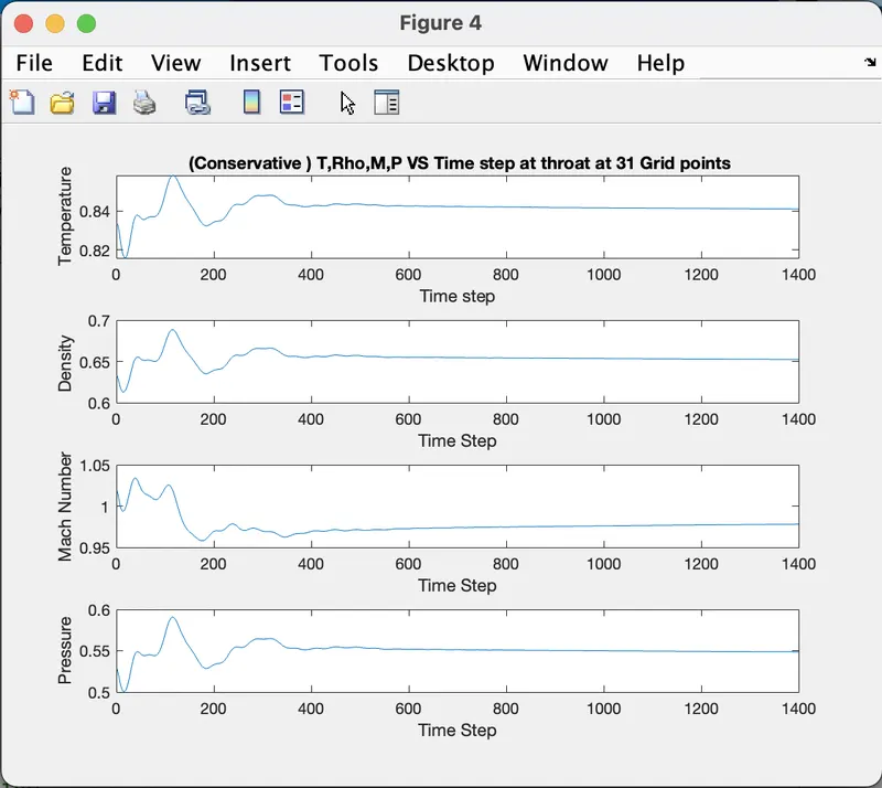
1. Time-wise variation of the primitive variable -

Conservative form -

Non-Conservative form -

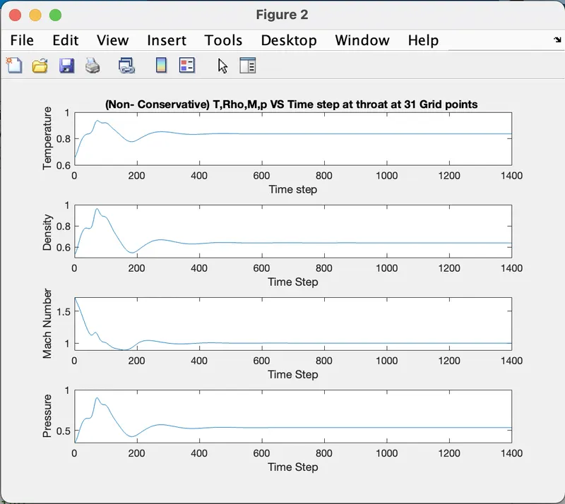
It is observed that Steady state results are obtaioned from 500 timestep onwards.

2. Steady-state distribution of primitive variables inside the nozzle -

Conservative form -

Non-Conservative form -

It is observed in the above two graphs as Velocity increases from inlet to outlet at the expense of pressure drop. Density and temperature drop from inlet to outlet as well.

3. Variation of Mass flow rate distribution inside the nozzle at different time steps during the time-marching process -

Conservative form -

Non-Conservative form -

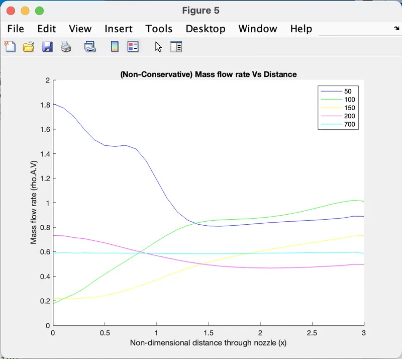
It is observed that conservative form seems to produce more consistent results when it comes to mass flow but in case of non-conservative graph, we see that results show huge variation near initial and final values.

4. Comparison of Normalized mass flow rate distributions of both forms -

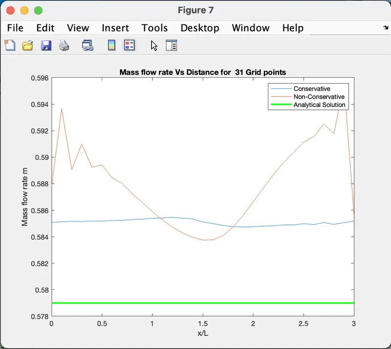
Observation -

Grid dependency is an important factor to determine whether the problem can be solved faster. So here we increased the Grid points from 31 to 61 is shown below.

It is clear from the below graphs that the values are almost same along all the Primitive Variables for both the forms even when the Grid points(n) is changed from 31 to 61 showcasing that it doesn't get affected by the increase of Grid points.

So it is conclude that the above problem is Grid Dependant.

Graphs for Grid Point 61 -