Week 3 - Solving second order ODEs

AIM - To solve a second order ode and to animate a simple pendulum.

Equaltion to solve the ODE function -

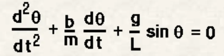
Theory -

ODE45 function - Ode45 function in matlab is used to solve differential equation using a numerical method. It takes 3 inputs as a function to be integrated, initial condition and time span.

%Sloving second order ODE (ode45)
%program animate a simple pendulum

clear 
close
clc

%given inputs
b = 0.05;       %damping coefficient
g = 9.81;       %g = gravity in m/s2,
l = 1;          %length = 1 m
m = 1;          %mass = 1 kg

%initial condition
theta_0 = [0;3];            %here initial displacement is 0 and velocity is 3m/s.

%time span
t_span = linspace(0,10,500);   

%solveing ODE
[t, results] = ode45(@(t,theta) ode_func(t,theta,b,g,l,m),t_span, theta_0);

%ploting 
plot(t,results(:,1))
hold on
plot(t,results(:,2))
ylabel('Plot')             %defining labels
xlabel('Time in sec')

% Using for loop to create animation of simple pendulum
ct=1;                      %counter 
theta_1 = results(:,1);
for i= 1:length(results(:,1))   %defining for loop

    %initializing co-ordinates
    x_start= 0;
    y_start= 0;
    theta_2 = theta_1(i);

    %final co-ordinates
    x_end = 1*sin(theta_2);
    y_end = -1*cos(theta_2);

    %ploting for animation
    figure(2)

    %base of pendulum
    plot([-1,1],[0,0], 'linewidth',5,'color','black')
    hold on

    %string of pendulum
    line([x_start x_end],[y_start y_end],'linewidth',4,'color','b')
    hold on

    %bob of pendulum
    plot(x_end,y_end,'marker','o','markersize', 24,'markerfacecolor','g')
    axis([-2 2 -2 2])
    pause(0.03)
    hold off
    M(ct)=getframe(gcf);
    ct=ct+1;
end

% creating animation from captured frames
 movie(M)
 videofile = VideoWriter('simple_pendulum.avi','uncompressed AVI');
 open(videofile);
 writeVideo(videofile,M);
 close(videofile);

 

Stepwise explaination -

1. providing inputs and the initial condition.

2. providing time span with number of intervals.

3. solving ODE function and plotting a graph of velocity and displacement.

4. Using 'for loop' for iteration, under which we are giving initial and final conditions.

5. Plotting the animation as figure(2) by configuring the base and the string length and the bob of the pendulum.

6. At the end, creating an animation/video file by using 'MOVIE' function by joining all the feames captured during the process.

%ode function code file

function [dtheta_dt] = ode_func(~,theta,b,g,l,m)
theta1 = theta(1);
theta2 = theta(2);
dtheta1_dt = theta2;
dtheta2_dt = -(b/m)*theta2 - (g/l)*sin(theta1);
dtheta_dt = [dtheta1_dt; dtheta2_dt];
end

This is a seperate function code file which we will call out in this code where ode function is defined by providing all the inputs from the main code.

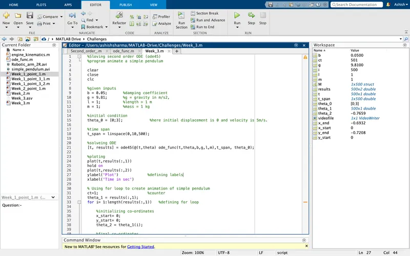
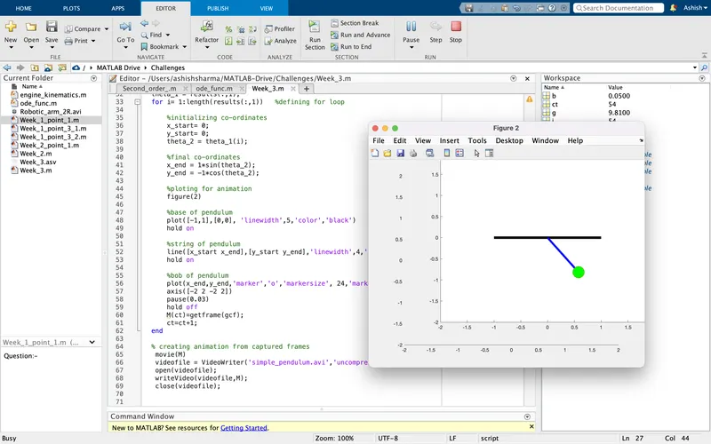
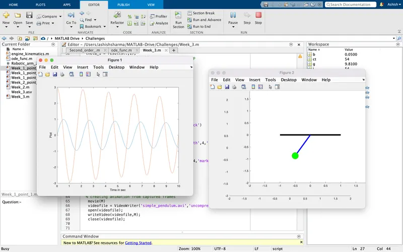
OUTPUT - the output is obtained as the graphical representation of velocity and displacement curve which is generated for a time span of 10sec. And aslo animated a simple pendulum out of that equation.

Youtube video link - https://youtu.be/JhwG4kA3R54

Conclusion - So, successfully completed the animation of simple pendulum by solving a second order ODE.