Week 7 - Simulation of a 1D Super-sonic nozzle flow simulation using Macormack Method
Objective:-
1) Steady-state distribution of primitive variables inside the nozzle
2) Time-wise variation of the primitive variables
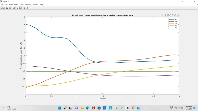
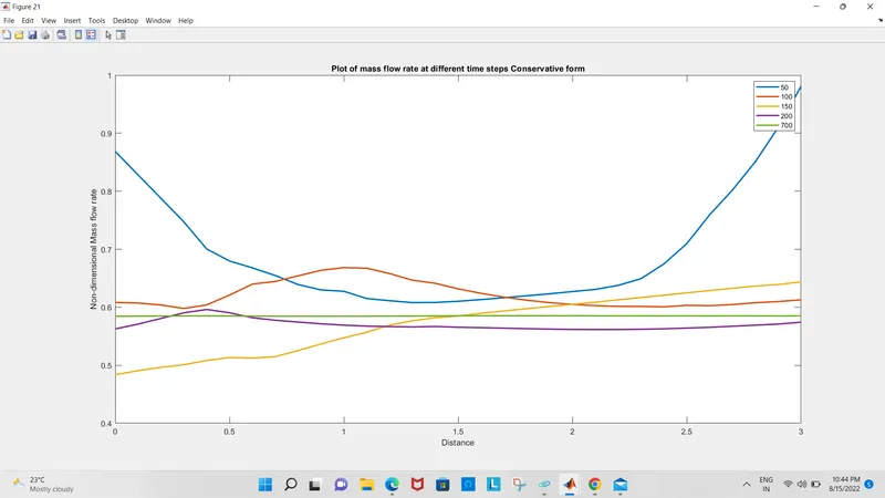
3) Variation of Mass flow rate distribution inside the nozzle at different time steps during the time-marching process
4) Comparison of Normalized mass flow rate distributions of both forms
THEORY:-
A nozzle is a device designed to control the direction or characteristics of a fluid flow (especially to increase velocity) as it exits (or enters) an enclosed chamber or pipe. A nozzle is often a pipe or tube of varying cross sectional area, and it can be used to direct or modify the flow of a fluid (liquid or gas). Nozzles are frequently used to control the rate of flow, speed, direction, mass, shape, and/or the pressure of the stream that emerges from them.
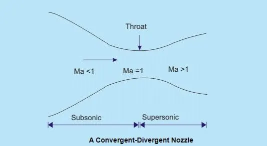
There are different types of nozzle But here in our project we uses a Convergent Divergent nozzle. This nozzle is used to obtain a supersonic stream starting from low speeds at the inlet. Then the Mach number should increase from Ma=0 near the inlet to Ma>1 at the exit. It is clear that the nozzle must converge in the subsonic portion and diverge in the supersonic portion. Such a nozzle is called a convergent-divergent nozzle.
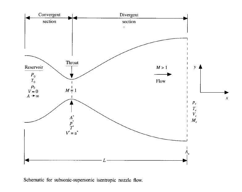
Here we are considering the steady,isentropic flow through a convergent-divergent nozzle as given below, The flow at the inlet to the nozzle comes from a reservoir where the pressure and temperature are denoted by P0andT0 P0andT0. The cross -sectional area of the reservior is large (A = ∞∞), and hence the velocity is very small (V=0). Thus P0andT0P0andT0 are the stagnation values, or total pressure and total temperature, respectively. The flow expands isentropically to supersonic speeds at the nozzle exit, where the exit pressure, temperature, velocity and Mach number are denoted by Pe,Te,VeandMePe,Te,VeandMe . The flow is locally subsonic in the convergent section of the nozzle, sonic at the throat and supersonic at the divergent section. The sonic flow (M=1) at the throat means that the local velocity at this location is equal to the local speed of sound. We denote the pressure, temperature, velocity, and area as P*,T*, V* (Which is equal to V* = a* (speed of sound)), and A*.
We assume that at a given section, where the cross-sectional area is A the flow properties are uniform across the section. Hence the area of the section changes as a function of distance along the nozzle x and therefore in reality the flow field is 2-dimensional, we make the assumption that the flow properties vary only with x, this is equal to assuming uniform flow properties across any given cross section. Such flow is defined as quasi-one-dimensional flow.
Setup followed to solve the 1D Super-sonic nozzle flow simulation using Macormack Method :-
1) The governing flow equations will be couched in terms of partial differential equation suitable for the time marching solution of quasi-one-dimensional flow
2) The finite-difference expressions pertaining to MacCormack's technique as applied to this problem will be set up.
3) Other details for the numerical solution (such as calculation of timestep and the treatment of boundary condition) will be formulated.
Step-1 - Governing equations
For Non-Conservative:-
* Continuity Equation

* Momentum Equation

*Energy Equation

For Conservative:-
* Continuity Equation
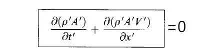
* Momentum Equation

*Energy Equation

Step-2- Finite difference expressions using MacCormack's explicit technique for the numerical solution
To implement a finite-difference solution, we divide the x-axis along the nozzle into a number of discrete grid points,
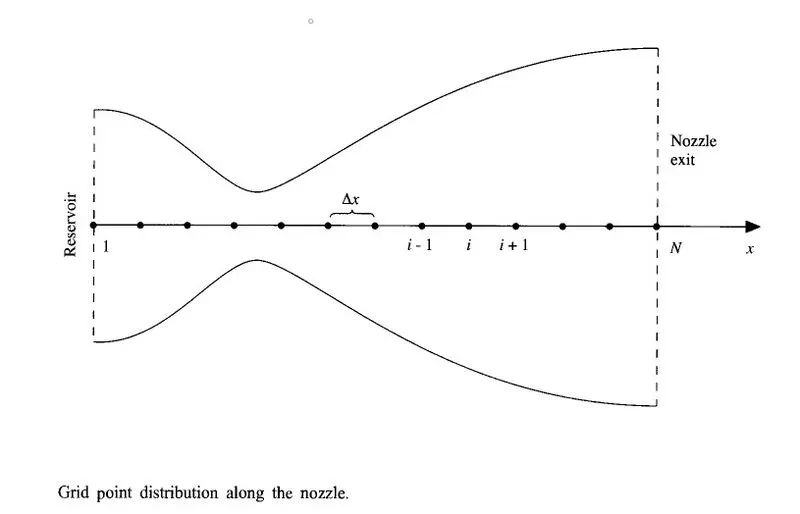
The first grid point, labeled as point 1, is assumed to be in the reservior. The points are evenly distributed along the x axis, with △x△x denoting the spacing between grid points. The last point, namely, that at the nozzle exit, is denoted by N; we have a total number od N grid points distributed along the axis. Point i is simply an arbitrary grid point, with points i-1 and i+1 as the adjacent points. MacCormack's technique is a predictor-corrector method. In the time marching approach, remember that we know the flow-field variables at time t , and we use the difference equations to solve explicitly for the variables at time t+△tt+△t
Non Conservasion form
First, we consider the predictor step, we set up the spatial derivatives as forwarding differences.
Continuity Equation:-

Momentum Equation:-

Energy Equation:-

Using the above values we will obtain the predicted values of ρρ, V, and T.
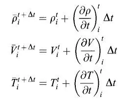
But these values are only First order accurate. So we do the corrector step to make it Second order accurate.
In the corrector step, we first obtain predicted values of the time derivative at time t+△tt+△t, (∂ρ∂t)t+△ti,j(∂ρ∂t)i,jt+△t , by substituting the predicted values of ρρ, u, and v into the right side of the continuity equation, replacing the spatial derivatives with rearward differences.
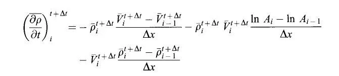
Likewise, momentum and energy equations will be,

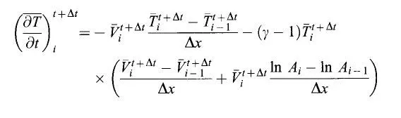
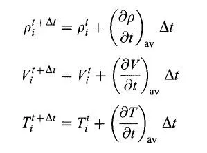
Using the above equations, the average time derivatives are
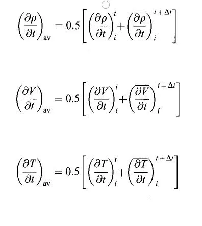
Then we can substitute the values into the below formula to find the corrected values of the flow-field variables at time t+△tt+△t
Conservation form
The equations for quasi-one-dimensional flow can be expressed in generic form. Let us define the elements of the solutions vector U, the flux vector F, and the source term J as follows
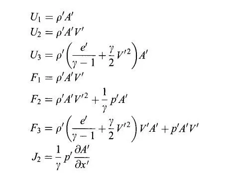
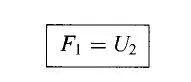
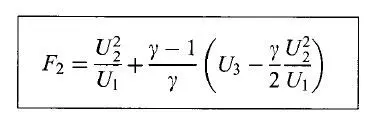
First we will find the source vectors with the above equations with initial condition, then with them we can find the flux vectors.
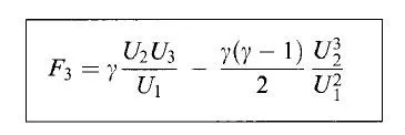
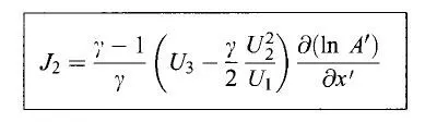
Predictor Step :-
Then we set up the spatial derivatives as forward differences .
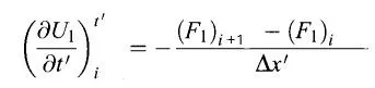

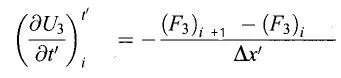
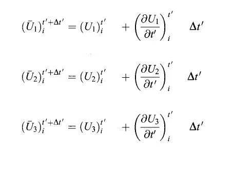
Then we find the predicted values of U1, U2 and U3
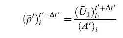
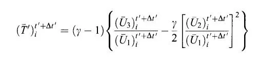
Using these values we will find the predicted values of the primitive variables
Now update the flux vector F1, F2, F3 with the new density , temperature and velocity.
Corrector Step :-
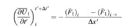
The predicted time derivatives of U1, U2 and U3 are obtained above. and Corrector time derivatives can be find using rearward differences for the x derivatives.


Then the average time derivatives are formed as follows :-
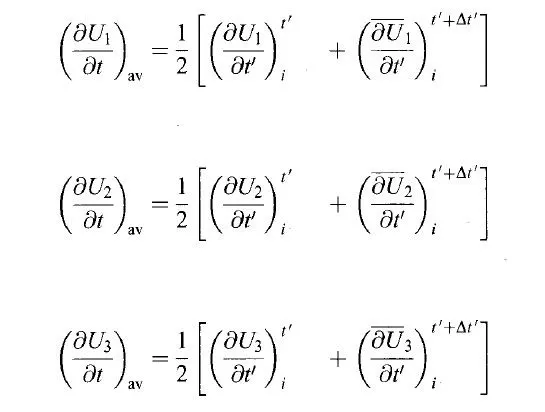
So, the final corrected values of U1, U2, U3 will become,
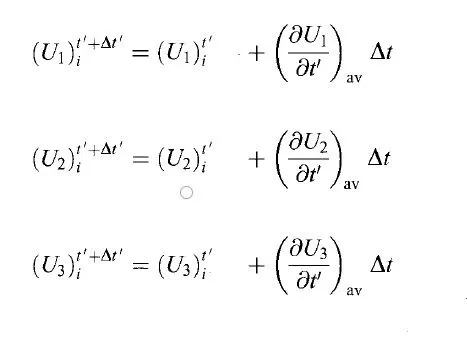
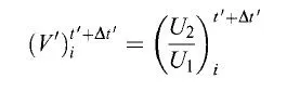
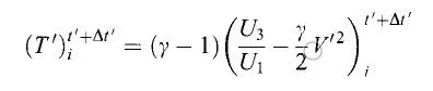
Finally the corrected values of the primitive variables are obtained by decoding U1, U2 and U3 obtained above.
(ρ')t'+△t'i=(U1)t'+△t'i(A)t'+△t'i(ρ′)it′+△t′=(U1)it′+△t′(A)it′+△t′
Step-3- Setting Time step calculation , initial and boundary conditions
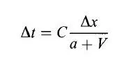
Time step can be calculated using the following formula :-
where,
C = Courant number
a = speed of sound
V= velocity
△x△x = Distance between to consecutive points.
Non Conservative form
Nozzle shape :-

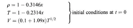
Initial conditions:-
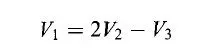
The boundary condition at Inlet:-
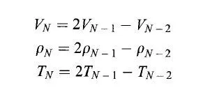
The boundary condition at the outlet
Conservative form
Nozzle shape:-
Initial condition:-
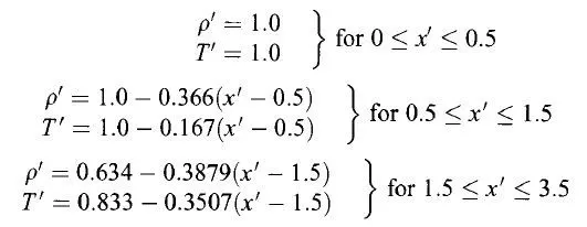
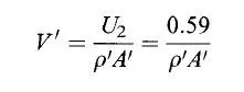
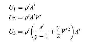
The boundary condition at inflow:-

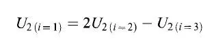
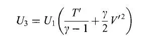
The boundary condition at outflow:-
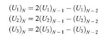
FOR NON-CONSERVATION FORM
MATLAB CODE
close all
clear all
clc

%input
n=input('Number of grid points :-');
nt=input('Number of time step:-');

% Non Conservative form
[rho,v,t,P,M,rho_t,v_t,t_t,P_t,M_t,x,a]=non_conservative(n,nt);

% Conservative form
[rho_c,v_c,t_c,P_c,M_c,rho_t_c,v_t_c,t_t_c,P_t_c,M_t_c,x,a]=conservative(n,nt)


% Plots for Non Conservative, Mach number , pressure and temperature Vs distance at 1400 time step
figure()
plot(x,M)
title_text=sprintf('Non conservative \n Mach number vs Distance (No. of Timestep=%d)',nt);
title(title_text)
xlabel('Distance')
ylabel('Mach number')


figure()
plot(x,P)
title_text=sprintf('Non conservative \n Pressure vs Distance (No. of Timestep=%d)',nt);
title(title_text)
xlabel('Distance')
ylabel('Pressure')

figure()
plot(x,rho)
title_text=sprintf('Non conservative \n Density vs Distance (No. of Timestep=%d)',nt);
title(title_text)
xlabel('Distance')
ylabel('Density')

figure()
plot(x,t)
title_text=sprintf('Non conservative \n Temperature vs Distance (No. of Timestep=%d)',nt);
title(title_text)
xlabel('Distance')
ylabel('Temperature')

% Plots for Conservative, Mach number , pressure and temperature Vs distance at 1400 time step

figure()
plot(x,M_c)
title_text=sprintf('Conservative \n Mach number vs Distance (No. of Timestep=%d)',nt);
title(title_text)
xlabel('Distance')
ylabel('Mach number')


figure()
plot(x,P_c)
title_text=sprintf('Conservative \n Pressure vs Distance (No. of Timestep=%d)',nt);
title(title_text)
xlabel('Distance')
ylabel('Pressure')

figure()
plot(x,rho_c)
title_text=sprintf('Conservative \n Density vs Distance (No. of Timestep=%d)',nt);
title(title_text)
xlabel('Distance')
ylabel('Density')

figure()
plot(x,t_c)
title_text=sprintf('Conservative \n Temperature vs Distance (No. of Timestep=%d)',nt);
title(title_text)
xlabel('Distance')
ylabel('Temperature')

% Plots for Non Conservative, Mach number , pressure and temperature Vs distance at Throat area


nt=(1:1400);

figure()
plot(nt,M_t)
title_text=sprintf('Non conservative \n Mach number vs Distance at Throat');
title(title_text)
xlabel('Distance')
ylabel('Mach number')

figure()
plot(nt,P_t);
title_text=sprintf('Non conservative \n Pressure vs Distance at Throat');
title(title_text)
xlabel('Distance')
ylabel('Pressure')
figure()
plot(nt,rho_t)
title_text=sprintf('Non conservative \n Density vs Distance at Throat');
title(title_text)
xlabel('Distance')
ylabel('Density')

figure()
plot(nt,t_t)
title_text=sprintf('Non conservative \n Temperature vs Distance at Throat');
title(title_text)
xlabel('Distance')
ylabel('Temperature')

% Plots for Conservative, Mach number , pressure and temperature Vs distance at Throat area


figure()
plot(nt,M_t_c)
title_text=sprintf('Conservative \n Mach number vs Distance at Throat');
title(title_text)
xlabel('Distance')
ylabel('Mach number')

figure()
plot(nt,P_t_c);
title_text=sprintf('Conservative \n Pressure vs Distance at Throat');
title(title_text)
xlabel('Distance')
ylabel('Pressure')
figure()
plot(nt,rho_t_c)
title_text=sprintf('Conservative \n Density vs Distance at Throat');
title(title_text)
xlabel('Distance')
ylabel('Density')

figure()
plot(nt,t_t_c)
title_text=sprintf('Conservative \n Temperature vs Distance at Throat');
title(title_text)
xlabel('Distance')
ylabel('Temperature')


% Mass flow rate distribution inside the nozzle

figure()
m=rho.*a.*v;
m_c=rho_c.*a.*v_c;
plot(x,m)
hold on
plot(x,m_c)
line([0 3],[0.579 0.579],'color','g')
title_text=sprintf('Mass Flow rate vs Distance');
title(title_text)
% axis([0 3 .578 .596])
xlabel('Distance')
ylabel('Mass Flow Rate')
legend('Non Conservative Form','Conservative form','Analytical form')Explanation:-
1) Here I have given code to input the number of grid points and a number of timesteps So that we can change the values as we want.
2) Then I have given functions for the Non-conservative form and Conservative Form
3) After that I have given codes to plot the graphs.
Function Code For Non-Conservative:-
function [rho,v,t,P,M,rho_t,v_t,t_t,P_t,M_t,x,a]=non_conservative(input1,input2)

%inputs
n=input1;
x= linspace(0,3,n);
dx=x(2)-x(1);

%Calculating initial profile

rho=1-0.3146*x;    %density
t=1-0.2314*x;      %temperature
v=(0.1+1.09*x).*t.^(1/2);  %velocity
a=1+(2.2*(x-1.5).^2);   %area
gamma=1.4;

% no. of timestep
nt=input2;

% time step
delta_t=0.5*(dx./((sqrt(t)+v)));
dt=min(delta_t);

% Time marching
for k=1:nt
    rho_old=rho;
    v_old=v;
    t_old=t;

    %Predictor Method
    for i=2:n-1
        dvdx=(v(i+1)-v(i))/dx;
        drhodx=(rho(i+1)-rho(i))/dx;
        dtdx=(t(i+1)-t(i))/dx;
        dlogadx=(log(a(i+1))-log(a(i)))/dx;

        %drho_dt_p(i)= -rho(i)*(v(i+1)-v(i))/dx-rho(i)*v(i)*(log(a(i+1))-log(a(i)))/dx-v(i)*(rho(i+1)-rho(i))/dx;

        %Continuity Equation
        drhodt_p(i)= -rho(i)*dvdx-rho(i)*v(i)*dlogadx-v(i)*drhodx;
        %Momentum Equation
        dvdt_p(i)= -v(i)*dvdx-(1/gamma)*(dtdx+(t(i)/rho(i))*drhodx);
        %Energy Equation
        dtdt_p(i)= -v(i)*dtdx-(gamma-1)*t(i)*(dvdx+v(i)*dlogadx);

    %Solution update
    rho(i)=rho(i)+drhodt_p(i)*dt;
    v(i)=v(i)+dvdt_p(i)*dt;
    t(i)=t(i)+dtdt_p(i)*dt;

    end


    %Corrector Method
    for j=2:n-1
        dvdx=(v(j)-v(j-1))/dx;
        drhodx=(rho(j)-rho(j-1))/dx;
        dtdx=(t(j)-t(j-1))/dx;
        dlogadx=(log(a(j))-log(a(j-1)))/dx;

        %Continuity Equation
        drhodt_c(j)= -rho(j)*dvdx-rho(j)*v(j)*dlogadx-v(j)*drhodx;
        %Momentum Equation
        dvdt_c(j)= -v(j)*dvdx-(1/gamma)*(dtdx+(t(j)/rho(j))*drhodx);
        %Energy Equation
        dtdt_c(j)= -v(j)*dtdx-(gamma-1)*t(j)*(dvdx+v(j)*dlogadx);
    end

    %Average Time derivatives
    rho_avg=0.5*(drhodt_p+drhodt_c);
    v_avg=0.5*(dvdt_p+dvdt_c);
    t_avg=0.5*(dtdt_p+dtdt_c);

    %Solution Updates
    for m=2:n-1
        rho(m)=rho_old(m)+rho_avg(m)*dt;
        v(m)=v_old(m)+v_avg(m)*dt;
        t(m)=t_old(m)+t_avg(m)*dt;
    end
    % Applying boundary condition

    %inlet
    v(1)=2*v(2)-v(3);
    %outlet
    v(n)=2*v(n-1)-v(n-2);
    rho(n)=2*rho(n-1)-rho(n-2);
    t(n)=2*t(n-1)-t(n-2);

    %Mach Number
    M=(v./sqrt(t));

    %Pressure
    P=rho.*t;

    % Throat datas
    throat= find(a==1);
    rho_t(k)=rho(throat);
    t_t(k)=t(throat);
    v_t(k)=v(throat);
    P_t(k)=P(throat);
    M_t(k)=M(throat);

    % mass flow rate
    mass = rho.*v.*a;

          %if else condition to plot the variation of non dimensional mass flow rate at specific time steps and plot the same
       if k == 50
          %plotting of mass flow rate at time step 50
          figure(20)
          plot(x,mass,'Linewidth', 2)
          hold on
      elseif k == 100
          %plotting of mass flow rate at time step 100
          plot (x,mass,'Linewidth', 2)
      elseif k==150
          %plotting of mass flow rate at time step 150
          plot(x,mass,'Linewidth', 2)
       elseif k==200
           %plotting of mass flow rate at time step 200
           plot (x,mass,'Linewidth', 2)
       elseif k==700
           %plotting of mass flow rate at time step 700
           plot (x,mass,'Linewidth', 2)
           title ('Plot of mass flow rate at different time steps Non conservative form')
           xlabel('Distance')
           ylabel('Non-dimensional Mass flow rate')
           legend ('50','100','150','200','700')
       end


end
end
1) In the funtion we have inputed the number of timestep and number of grid points.
2) with these values the initial condition is calculated
3) Then using MacCormack's Technique we will find the predictor and corrector values
4) We get the new solution
5) Apply the Boundary conditions for calculating the next timestep
6) Then the for loop will goes on til the given value.
function [rho_c,v_c,t_c,P_c,M_c,rho_t_c,v_t_c,t_t_c,P_t_c,M_t_c,x,a]=conservative(input1,input2)

%inputs
n=input1;
x= linspace(0,3,n);
dx=x(2)-x(1);

%Calculating initial profile


%Desity and Temperature with respect to x

for i=1:length(x)
    if (x(i)<=3.5)
        rho= 0.634-0.3879*(x-1.5);   % density
        t=0.833-0.3507*(x-1.5);    % Temperature
    end
end

    for i=1:length(x)
    if (x(i)<=1.5)
        rho(i)=1.0-0.366*(x(i)-0.5)  % density
        t(i)=1.0-0.167*(x(i)-0.5)    % Temperature
    end
    end

    for i=1:length(x)
    if (x(i)<=0.5)
        rho(i)=1.0   % density
        t(i)=1.0    % Temperature
    end
end

a=1+(2.2*(x-1.5).^2);    % area
v=(.59)./(rho.*a);      % velocity
gamma=1.4;

% no. of timestep
nt=input2;

% time step
delta_t=0.5*(dx./((sqrt(t)+v)));
dt=min(delta_t);

    % Solution Vector
    U1=rho.*a;
    U2=rho.*a.*v;
    U3=rho.*((t./(gamma-1))+(gamma/2).*v.^2).*a;

for k=1:nt
    U1_old=U1;
    U2_old=U2;
    U3_old=U3;


    %Flux Vector

    F1=U2;
    F2=((U2.^2)./U1)+((gamma-1)/gamma)*(U3-(gamma/2)*(((U2).^2)./U1));
    F3=(((gamma)*(U2.*U3))./U1)-(((gamma*(gamma-1))/2)*((U2.^3)./U1.^2));


    %Predictor Step
  for j=2:n-1

    J2(j)=(1/gamma)*rho(j)*t(j)*((a(j+1)-a(j))/dx);

    dU1dt_p(j)=-((F1(j+1)-F1(j))/dx);
    dU2dt_p(j)=-((F2(j+1)-F2(j))/dx)+J2(j);
    dU3dt_p(j)=-((F3(j+1)-F3(j))/dx);


    U1(j)=U1_old(j)+(dU1dt_p(j))*dt;
    U2(j)=U2_old(j)+(dU2dt_p(j))*dt;
    U3(j)=U3_old(j)+(dU3dt_p(j))*dt;
  end

  %Solution Update
    rho=(U1./a);
    v=(U2./U1);
    t= (gamma-1)*((U3./U1)-(gamma/2)*(v).^2);


  %Updating F1,F2,F3


    %Flux Vector

    F1=U2;
    F2=((U2.^2)./U1)+((gamma-1)/gamma)*(U3-(gamma/2)*(((U2).^2)./U1));
    F3=(((gamma)*(U2.*U3))./U1)-(((gamma*(gamma-1))/2)*((U2.^3)./U1.^2));

    %Corrector Step
  for m=2:n-1

    J2(m)=(1/gamma)*rho(m)*t(m)*((a(m)-a(m-1))/dx);

    dU1dt_c(m)=-((F1(m)-F1(m-1))/dx);
    dU2dt_c(m)=-((F2(m)-F2(m-1))/dx)+J2(m);
    dU3dt_c(m)=-((F3(m)-F3(m-1))/dx);

  end

  % Average Time derivatives

    dU1dt_avg=(1/2)*(dU1dt_p+dU1dt_c);
    dU2dt_avg=(1/2)*(dU2dt_p+dU2dt_c);
    dU3dt_avg=(1/2)*(dU3dt_p+dU3dt_c);

  for i=2:n-1


      U1(i)=U1_old(i)+(dU1dt_avg(i)*dt);
      U2(i)=U2_old(i)+(dU2dt_avg(i)*dt);
      U3(i)=U3_old(i)+(dU3dt_avg(i)*dt);


  end

      %Solution Update
      rho_c=U1./a;
      v_c=(U2./U1);
      t_c=(gamma-1)*((U3./U1)-(gamma/2)*(U2./U1).^2);


        %Defining Inletflow Boundary conditions
        U1(1)=rho_c(1)*a(1);
        U2(1) = 2*U2(2)-U2(3);
        v(1)=U2(1)/U1(1);
        U3(1) = U1(1)*(t(1)/(gamma-1)+(gamma/2)*v(1)^2);


        %Defining outflow Boundary conditions

        U1(n)=2*U1(n-1)-U1(n-2);

        U2(n)=2*U2(n-1)-U2(n-2);

        U3(n)=2*U3(n-1)-U3(n-2);


    %Mach Number
    M_c=(v_c./sqrt(t));

    %Pressure
    P_c=rho_c.*t_c;

    % Throat datas
    throat= find(a==1);
    rho_t_c(k)=rho_c(throat);
    t_t_c(k)=t_c(throat);
    v_t_c(k)=v_c(throat);
    P_t_c(k)=P_c(throat);
    M_t_c(k)=M_c(throat);

    % mass flow rate
    mass = rho.*v.*a;


          %if else condition to plot the variation of non dimensional mass flow rate at specific time steps and plot the same
       if k == 50
          %plotting of mass flow rate at time step 50
          figure(21)
          plot(x,mass,'Linewidth', 2)
          hold on
      elseif k == 100
          %plotting of mass flow rate at time step 100
          plot (x,mass,'Linewidth', 2)
      elseif k==150
          %plotting of mass flow rate at time step 150
          plot(x,mass,'Linewidth', 2)
       elseif k==200
           %plotting of mass flow rate at time step 200
           plot (x,mass,'Linewidth', 2)
       elseif k==700
           %plotting of mass flow rate at time step 700
           plot (x,mass,'Linewidth', 2)

           title ('Plot of mass flow rate at different time steps Conservative form')
           xlabel('Distance')
           ylabel('Non-dimensional Mass flow rate')
           legend ('50','100','150','200','700')
       end


end
end
1) The convective funtion will also be the same as non-convective function.
2)We have inputed the number of timestep and number of grid points.
3) With these values the initial condition is calculated
4) Then using MacCormack's Technique we will find the predictor and corrector values
5) We get the new solution
6) Apply the Boundary conditions for calculating the next timestep
7) Then the for loop will go on til the given value.
Result:-
Non-Conservative:-
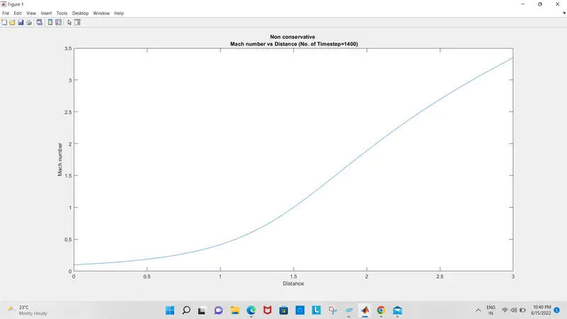
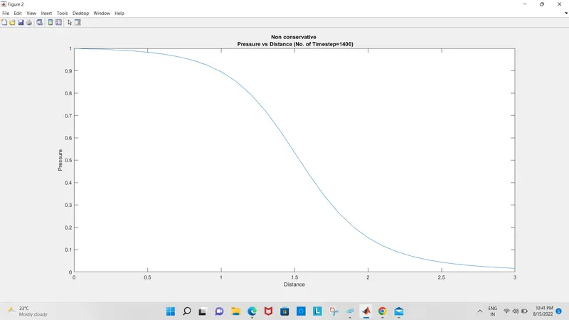
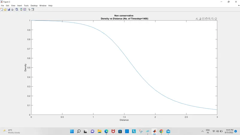
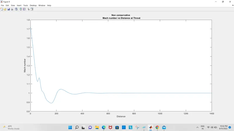
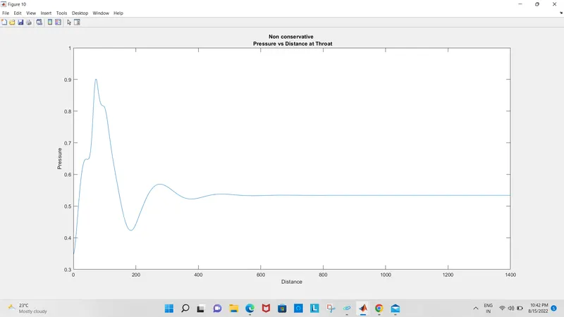
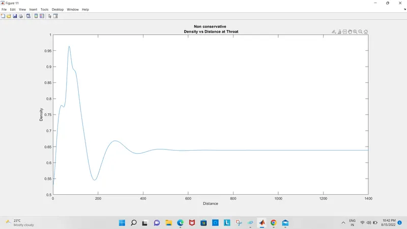
CONSERVATIVE:
Observations:-
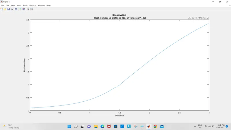
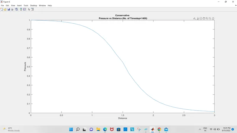
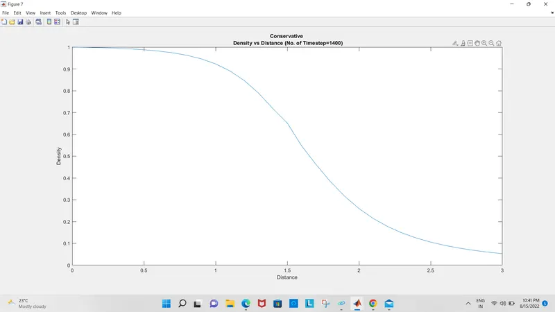
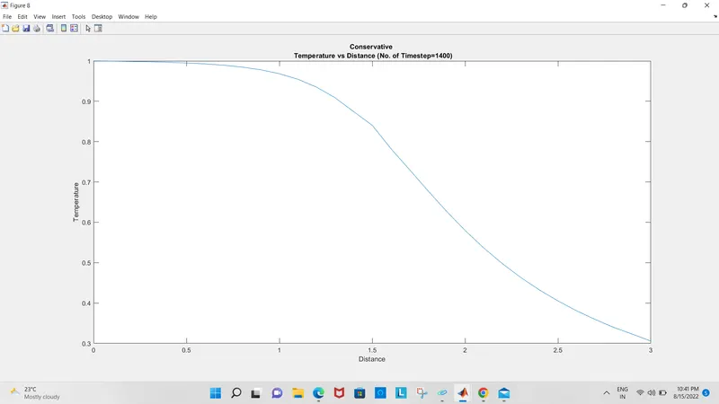
1) When we go through the graphs of the Distribution of primitive variables inside the nozzle, we can see that as we move from the inlet to outlet the mach number goes on increaseing. At the inlet Mach number will be less than 1, at the throat the mach number will be equal to 1 and at the outlet the mach number will be greater than 1. At the convergeing section the velocity will be less but velocity above mach number equal to 1 increases as the pipe cross section increases. Energy is created from the heat and pressure of the fluid, as velocity increases the temperature and pressure decreases. As the pressure decreases the density also decreases.
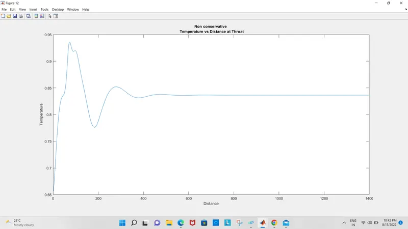
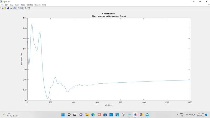
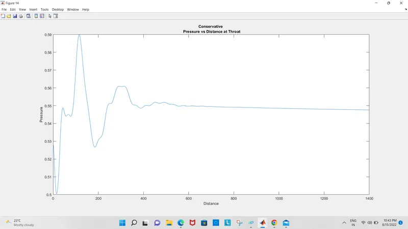
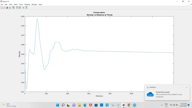
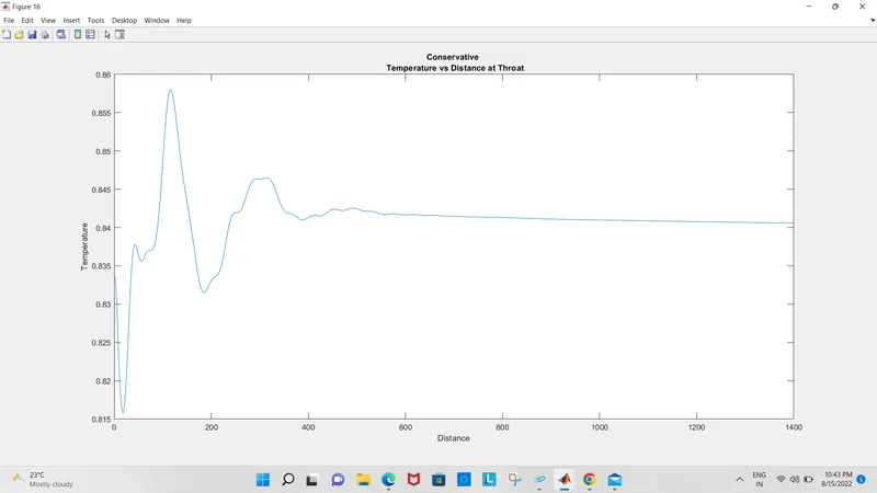
2) Looking at pressure, density , temperature and mach number at the nozzle throat plotted verse the number of time steps we can see that the largest changes take place at the early times after which the final,steady state value is approched. At early times, the time derivatives are large and they oscillate in value. These oscillations are associated with various unsteady compression and expansion wavws which propagate through the nozzle during the transient process. Later the time derivatives rapidly grow small over a finite number of timesteps.
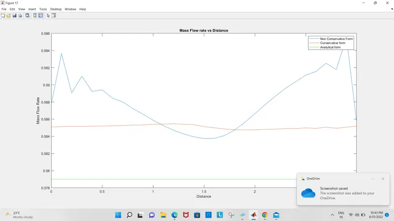
3)While comparing the steady state variation of the mass flow obtained with the non-conservation and conservation form of the governing equation we can see that conservation form of the equation is much more satisfactory than that obtained from the non conservation form. The conservation form gives a distribution that is much closer to being a constant. But the non conservation results have a sizeable variation, with some false oscillations at the both the inflow and outflow boundaries. Also the conservation form is much more closser to the exact analytical solution.
Conclusion :-
1) Better mass flow distribution is done in conservation form.
2) Non-conservation form is better for programming convenience because they are solved in term of primitive variables and their values are obtained directly. But in conservation form equation are expressed in terms of flux variables and first solve solution vector then the primitive variables which makes things complex.
3) For accuracy also non-conservative is better due to the direct calculation of primitive variables. While in conservation form primitive variables are calculated indirectly from flux variables. Increased number of calculations will lead to more errors. This is the case when we take primitive valrables. But if we are taking Flux variables conservation form is better.
4) In non conservation form behavior of the residuals are good as compare to conservation form. The residuals decays faster in non conservation form when compared to conservation form. The amount by which the residual decay is often used as an index 'quality' of the numerical algoritm. so the non conservation form is better.
5) The primitive variables converge to a numerical steady-state faster when using the non-conservation form.Because the dependent variables are primitive in non-conservation forms but not in conservation form, this might be the cause for that. Thus simulation time for the non-conservation form is shorter than the conservation form.