Week 7 - Simulation of a 1D Super-sonic nozzle flow simulation using Macormack Method

Aim:

To simulate the isentropic flow through a quasi 1D subsonic-supersonic nozzle & solve the conservation and non-conservation forms of the governing equations using the MacCormack's technique.

To plot the following graphs

1. Steady-state distribution of primitive variables inside the nozzle
2. Time-wise variation of the primitive variables
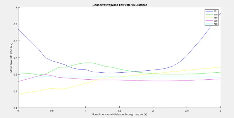
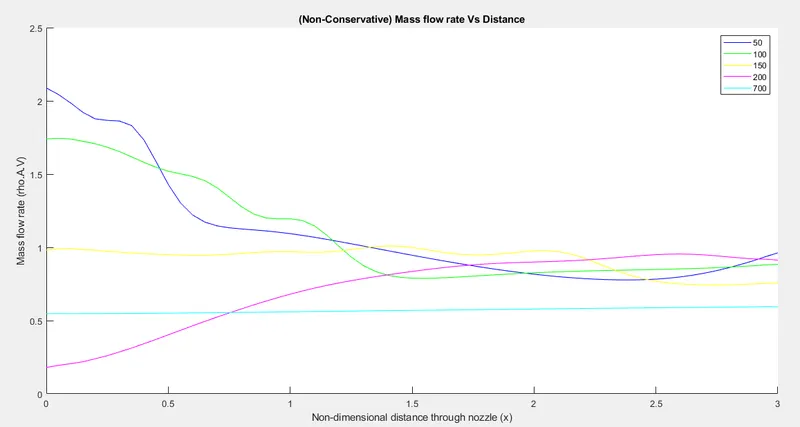
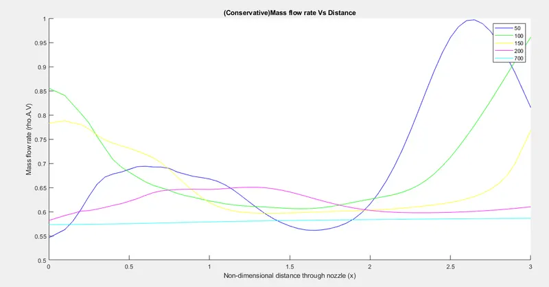
3. Variation of Mass flow rate distribution inside the nozzle at different time steps during the time-marching process
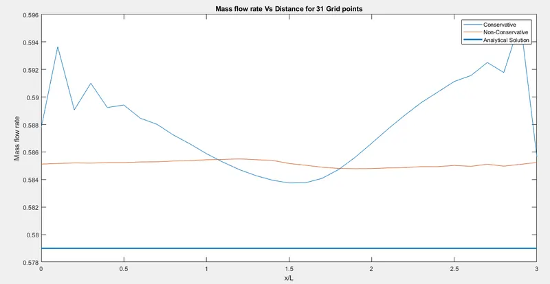
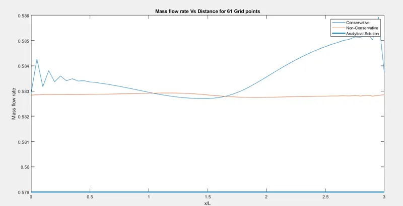
4. Comparison of Normalized mass flow rate distributions of both forms

Theory

A convergent divergent nozzle is described in the problem, where inlet is subsonic and at the outlet velocity is subsonic.

At the throat we are assuming a mach number of 1.

The convergence(subsonic) section connected with reservoir, here mach number is less than one. At throat area, the thermodynamic properties will become critical property as Mach number equal to 1. The sonic flow at the throat means that the local velocity at this point is equal to the local speed of sound and at divergence section(supersonic) the flow expands isentropically to supersonic speed at the nozzle exit. The corresponding notations are clearly written in the figure itself.

The flow is locally subsonic in the convergence section of the nozzle, sonic at the throat and supersonic at the divergence section.

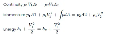
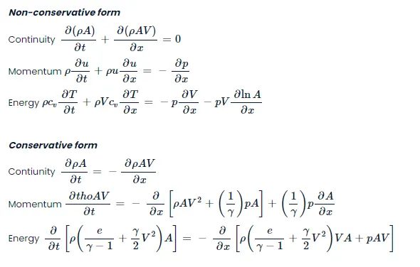
The governing continuity, momentum and energy equation for the quasi 1D steady isentropic flow can be expressed as

Steps for solving the Nozzle flow problem

Meshing

The given 1D domain is divided into n number of elements. For Nozzle flow problem the length of nozzle is chosen as 3 and the length is divided into 30 elements.

Discretization

The PDE is discretized and solved for the points in the domain. Maccormack method is used for discretizing the equation. Maccormack method gives better results for the hyperbolic equation and it is also called as a shock-capturing method. These methods can provide stable solutions in the presence of shock. Hence they are used in nozzle flow problems. In Maccormack method combination of both forward and backward differencing schemes can be used to solve for the primitive variables. Non-conservative and conservative form of governing equations are solved by using this method

The time step used for the simulation is

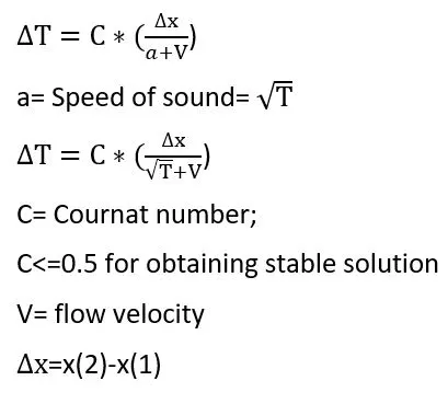
The minimum value of t is used such that the time marching solution is following the actual unsteady flow variation that exists in nature.

Steps involved in Maccormack method

• Predictor step(forward differencing)
• Solution update
• Corrector step( Backward differencing)
• Determining the average of the time derivative
• Final solution update

Non-conservative form of Governing equation

In the non-conservative form of governing equation the continuity, momentum and energy equations can be discretized directly to obtain the primitive variables such as density, velocity and temperature.

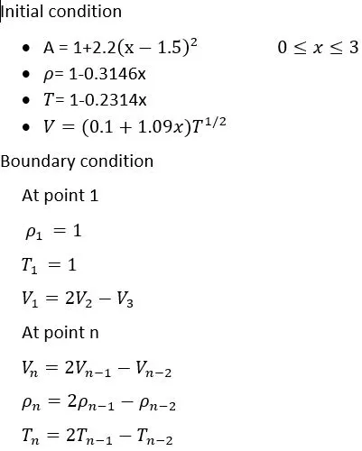
Main code

clear all

close all

clc

%Number of nodes

n=31;

x=linspace(0,3,n);

gamma=1.4;

dx=x(2)-x(1);

%area

a=1+(2.2*(x-1.5).^2);

% timestep

nt=2000;

% Non -conservative

[rho,v,t,M,p,m,p_t,rho_t,t_t,M_t]=non_conservative(n,nt);

%Conservative

[rho_c,v_c,t_c,M_c,p_c,m_c,p_tc,rho_tc,t_tc,M_tc]= conservative(n,nt);

% Non -conservative

% To plot variables Vs distance

figure(1)

subplot (4,1,1)

plot(x,M)

title_text=sprintf('(Non-Conservative method;No. of time steps = 2000');

title(title_text)

xlabel('Distance(m)')

ylabel('Mach number')

hold on

subplot(4,1,2)

plot(x,p)

xlabel('Distance(m)')

ylabel('Pressure(bar)')

hold on

subplot(4,1,3)

plot(x,rho)

xlabel('Distance(m)')

ylabel('Density(kg/m^3)')

hold on

subplot(4,1,4)

plot(x,t)

xlabel('Distance(m)')

ylabel('Temperature(k)')

hold on

% To plot variables at time step

figure(2)

nt=1:2000 ;

subplot(4,1,1)

plot (nt,t_t)

title('Non-Conservative method;No. of time steps = 2000')

xlabel('Time step(s)')

ylabel('Temperature(k)')

hold on

subplot(4,1,2)

plot(nt,rho_t)

xlabel('Time Step(s)')

ylabel('Density(kg/m^3) ')

hold on

subplot(4,1,3)

plot(nt,M_t)

xlabel('Time Step(s)')

ylabel('Mach Number')

hold on

subplot(4,1,4)

plot(nt,p_t)

xlabel('Time Step(s)')

ylabel('Pressure(bar)')

hold on

% Conservative

nt=2000 ;

figure(3)

subplot(4,1,1)

plot(x,M_c)

title('Conservative method;No. of time steps = 2000')

xlabel('Distance(m)')

ylabel('Mach number')

hold on

subplot(4,1,2)

plot(x,p_c)

xlabel('Distance(m)')

ylabel('Pressure(bar)')

hold on

subplot(4,1,3)

plot(x,rho_c)

xlabel('Distance(m)')

ylabel('Density(kg/m^3)')

hold on

subplot(4,1,4)

plot(x,t_c)

xlabel('Distance(m)')

ylabel('Temperature(k)')

hold on

figure(4)

nt=1:1400 ;

subplot(4,1,1)

plot (nt,t_tc)

title_text=('Conservative method;No. of time steps = 2000')

title(title_text)

xlabel('Time step(s)')

ylabel('Temperature(k)')

hold on

subplot(4,1,2)

plot(nt,rho_tc)

xlabel('Time Step(s)')

ylabel('Density(kg/m^3) ')

hold on

subplot(4,1,3)

plot(nt,M_tc)

xlabel('Time Step(s)')

ylabel('Mach Number')

hold on

subplot(4,1,4)

plot(nt,p_tc)

xlabel('Time Step(s)');

ylabel('Pressure(bar)');

hold on

figure(7)

plot(x,m_c)

hold on

plot(x,m)

line([0 3],[0.579 0.579],'linewidth',2);

title_text=sprintf( 'Mass flow rate Vs Distance for %d Grid points',n);

title(title_text);

legend ('Conservative','Non-Conservative', 'Analytical Solution');

xlabel('x/L');

ylabel('Mass flow rate');

Function : Non- conservative method

function[rho_c,v_c,t_c,M_c,p_c,m_c,p_tc,rho_tc,t_tc,M_tc]= conservative(n,nt)

x=linspace(0,3,n);

gamma=1.4;

dx=x(2)-x(1);

%area

a=1+(2.2*(x-1.5).^2);

for i=1:length(x)

if (x(i)>=0)&&(x(i)<=0.5)

rho(i)=1;

t(i)=1;

elseif (x(i)>=.5)&&(x(i)<=1.5)

rho(i)=1-.366.*(x(i)-0.5);

t(i)=1-.167.*(x(i)-0.5);

else

rho(i)=.634-.3879.*(x(i)-1.5) ;

t(i)=.833-.3507.*(x(i)-1.5);

end

end

a=1+(2.2*(x-1.5).^2);

v=(0.59)./(rho.*a);

U1=rho.*a;

U2=rho.*a.*v ;

U3= rho.*((t./(gamma-1)) + ((gamma/2).*v.^2)).*a;

delta_t= 0.5*(dx./(sqrt(t)+v));

dt=min(delta_t);

for k=1:nt

U1_old=U1;

U2_old=U2;

U3_old=U3;

F1=U2;

F2=((U2.^2)./U1)+((gamma-1)/gamma)*(U3-(gamma/2)*((U2.^2)./U1));

F3=(gamma*(U2.*U3)./U1)-((gamma*(gamma-1))/2)*((U2.^3)./(U1.^2));

%% Predictor

for j=2:n-1

J(j)=(1/gamma)*rho(j)*t(j)*((a(j+1)-a(j))/dx);

dU1dt_p(j)= -((F1(j+1)-F1(j))/dx);

dU2dt_p(j)=-((F2(j+1)-F2(j))/dx)+J(j) ;

dU3dt_p(j)= -((F3(j+1)-F3(j))/dx);

U1(j)=U1_old(j)+(dU1dt_p(j))*dt;

U2(j)=U2_old(j)+(dU2dt_p(j))*dt;

U3(j)=U3_old(j)+(dU3dt_p(j))*dt;

end

rho=U1./a ;

v= U2./U1;

t=(gamma-1)*((U3./U1)-((gamma/2)*(v.^2)));

% for i=1:length(n)

% delta_t(i)= 0.5*(dx(i)/sqrt(t(i))*v(i));

% end

% dt=min(delta_t);

%Update

%

% F1=U2;

% F2=U2.^2./U1+((gamma-1)/gamma)*(U3-(gamma/2).*(U2.^2./U1));

% F3=((gamma*U3.*U2)/U1)-((gamma*(gamma-1)/2)*(U2.^3./U1.^2));

F1=U2;

F2=((U2.^2)./U1)+((gamma-1)/gamma)*(U3-(gamma/2)*(((U2).^2)./U1));

F3=(((gamma)*(U2.*U3))./U1)-(((gamma*(gamma-1))/2)*((U2.^3)./U1.^2));

% corrector

for q=2:n-1

J(q)=(1/gamma)*rho(q)*t(q)*((a(q)-a(q-1))/dx)

dU1dt_c(q)= -(F1(q)-F1(q-1))/dx;

dU2dt_c(q)=-((F2(q)-F2(q-1))/dx)+J(q) ;

dU3dt_c(q)= -(F3(q)-F3(q-1))/dx;

end

dU1dt_av= 0.5*(dU1dt_p+dU1dt_c);

dU2dt_av=0.5*(dU2dt_p+dU2dt_c);

dU3dt_av=0.5*(dU3dt_p+dU3dt_c);

for m=2:n-1

U1(m)=U1_old(m)+(dU1dt_av(m)*dt);

U2(m)=U2_old(m)+(dU2dt_av(m)*dt);

U3(m)=U3_old(m)+(dU3dt_av(m)*dt);

end

%Defining Inletflow Boundary conditions

U1(1)=rho(1)*a(1);

U2(1) = 2*U2(2)-U2(3);

v(1)=U2(1)/U1(1);

U3(1) = U1(1)*(t(1)/(gamma-1)+(gamma/2)*v(1)^2);

%Defining outflow Boundary conditions

U1(n)=2*U1(n-1)-U1(n-2);

U2(n)=2*U2(n-1)-U2(n-2);

U3(n)=2*U3(n-1)-U3(n-2);

rho=U1./a;

v=(U2./U1);

t=(gamma-1)*((U3./U1)-(gamma/2)*(U2./U1).^2);

%Mach Number

M=(v./sqrt(t));

%Pressure

p=rho.*t;

% Mass flow rate

m=rho.*v.*a;

throat=find(a==1);

p_t(k)=p(throat);

rho_t(k)=rho(throat) ;

t_t(k)=t(throat);

M_t(k)=M(throat);

% m_t(k)=m(throat);

figure(6)

hold on

if k==50

plot(x,m,'b')

elseif k==100

plot(x,m,'g')

elseif k==150

plot(x,m,'y')

elseif k==200

plot(x,m,'m')

elseif k==700

plot(x,m,'c')

title('(Conservative)Mass flow rate Vs Distance')

legend('50','100','150','200','700')

xlabel('Non-dimensional distance through nozzle (x)')

ylabel('Mass flow rate (rho.A.V)')

end

end

rho_c=rho;

v_c=v;

t_c=t;

M_c=M;

p_c=p;

m_c=m;

p_tc=p_t;

rho_tc=rho_t;

t_tc=t_t;

M_tc=M_t;

%m_tc=m_t;

end

Function - Conservative method

function[rho,v,t,M,p,m,p_t,rho_t,t_t,M_t]= non_conservative(n,nt)

x=linspace(0,3,n);

gamma=1.4;

dx=x(2)-x(1);

%area

a=1+(2.2*(x-1.5).^2);

%calculate initial profile

rho=1-0.3146*x;

%temperature

t=1-0.2314*x;

v=(.1+1.09*x).*t.^0.5;

%area

a=1+2.2*(x-1.5).^2;

%timesteps

nt=1400;

dt=0.02;

delta_t= 0.5*(dx./(sqrt(t)+v));

dt=min(delta_t);

% % Outer time loop

for k=1:nt

% Predictor

rho_old=rho;

v_old=v;

t_old=t;

for j=2:n-1

%drho_dt_p=

dvdx=(v(j+1)-v(j))/dx;

drhodx=(rho(j+1)-rho(j))/dx;

dtdx=(t(j+1)-t(j))/dx;

dlogadx=(log(a(j+1))-log(a(j)))/dx;

%Continuity equation

drhodt_p(j)=-rho(j)*dvdx -rho(j)*v(j)*dlogadx-v(j)*drhodx;

%Momentum Equation

dvdt_p(j)= -v(j)*dvdx - ((1/gamma)*(dtdx + (t(j)/rho(j)*drhodx)));

%Energy Equation

dTdt_p(j)= -v(j)*dtdx-(gamma-1)*t(j)*(dvdx+v(j)*dlogadx);

%Solution Update

v(j)=v(j)+dvdt_p(j)*dt;

rho(j)=rho(j)+drhodt_p(j)*dt;

t(j)=t(j)+dTdt_p(j)*dt;

end

% Corrector Method

for j=2:n-1

%drho_dt_p=

dvdx=(v(j)-v(j-1))/dx;

drhodx=(rho(j)-rho(j-1))/dx;

dtdx=(t(j)-t(j-1))/dx;

dlogadx=(log(a(j))-log(a(j-1)))/dx;

%Continuity equation

drhodt_c(j)=-rho(j)*dvdx -rho(j)*v(j)*dlogadx-v(j)*drhodx;

%Momentum Equation

dvdt_c(j)= -v(j)*dvdx - ((1/gamma)*(dtdx + (t(j)/rho(j)*drhodx)));

%Energy Equation

dTdt_c(j)= -v(j)*dtdx-(gamma-1)*t(j)*(dvdx+v(j)*dlogadx);

% %Solution Update

% v(j)=v(j)+dvdt_p(j)*dt;

% rho(j)=rho(j)+drhodt_p(j)*dt;

% t(j)=t(j)+dTdt_p(j)*dt;

end

% Compute the average

drhodt_a= 0.5 *(drhodt_p+drhodt_c)

dvdt_a= 0.5*(dvdt_p+dvdt_c)

dTdt_a=0.5*(dTdt_p+dTdt_c)

for i=2:n-1

% Final solution update

v(i)=v_old(i)+dvdt_a(i)*dt;

rho(i)=rho_old(i)+drhodt_a(i)*dt;

t(i)=t_old(i)+dTdt_a(i)*dt;

end

% Apply Boundary COndition

% Inlet

v(1)=2*v(2)-v(3);

%outlet

v(n)=2*v(n-1)-v(n-2);

t(n)=2*t(n-1)-t(n-2);

rho(n)=2*rho(n-1)-rho(n-2);

% mach number

M=(v./sqrt(t));

% Density

p=rho.*t ;

% Mass flow

m=rho.*v.*a;

throat=find(a==1);

p_t(k)=p(throat);

rho_t(k)=rho(throat) ;

t_t(k)=t(throat);

M_t(k)=M(throat);

% m_t(k)=M(throat);

figure(5)

hold on

if k==50

plot(x,m,'b')

elseif k==100

plot(x,m,'g')

elseif k==150

plot(x,m,'y')

elseif k==200

plot(x,m,'m')

elseif k==700

plot(x,m,'c')

title('(Non-Conservative) Mass flow rate Vs Distance')

legend('50','100','150','200','700')

xlabel('Non-dimensional distance through nozzle (x)')

ylabel('Mass flow rate (rho.A.V)')

end

end

end

Result

Here we can observe that as X varies from 0 to 3m

Velocity increases

Pressurre decreases

Density decreases

Temperature decreases

At the throat Mach number 1 can be observed

In time step vs different functions, we can see that almost upto an iteration of 400 values were fluctuating,but after that the solution started converging to a stable value

Here we can observe that as X varies from 0 to 3m

Velocity increases

Pressurre decreases

Density decreases

Temperature decreases

At the throat Mach number 1 can be observed

In conservative method.solution seems to be converged well before 400 iterations, almost around 300 iterations

Now taking no. of grid points as 91

Mach number, pressure, density and temperature looks smooth and similiar to results from 31 grid points

Here it took more number of iterations to reach convergence

Here in conservative method,flow got stabilised well before than non-conservative method, flow is not smooth comparatively

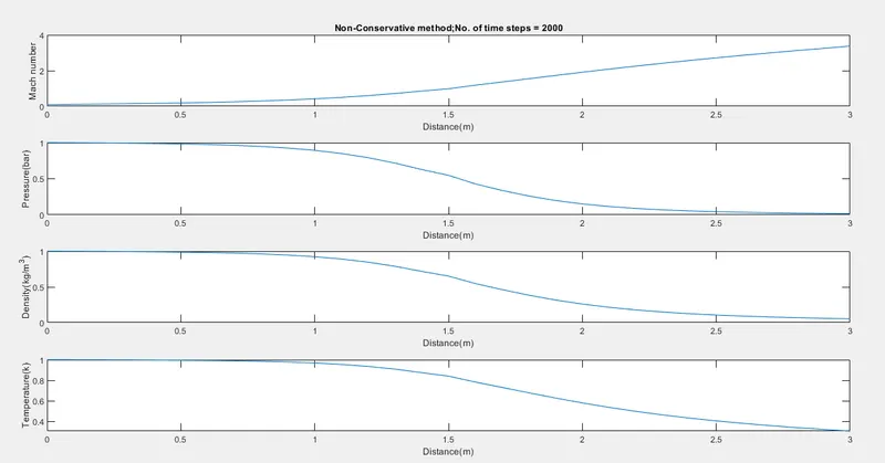
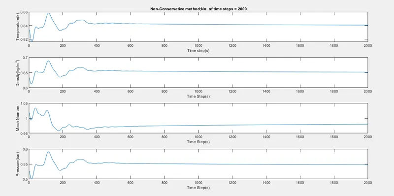
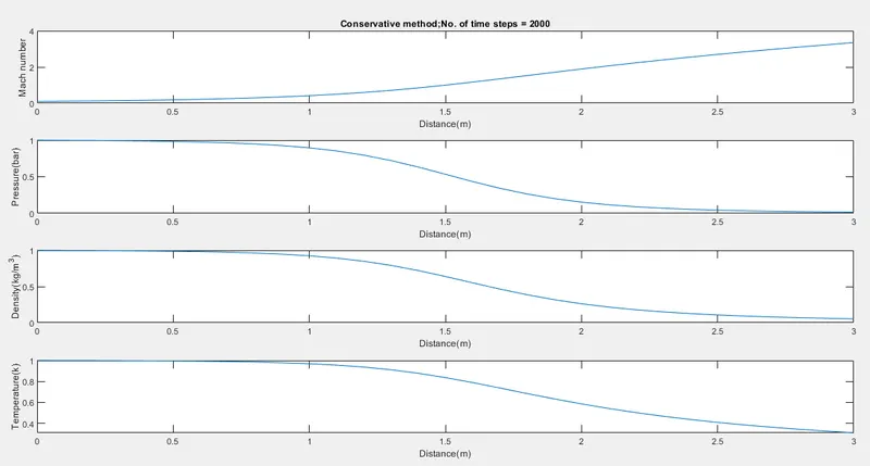
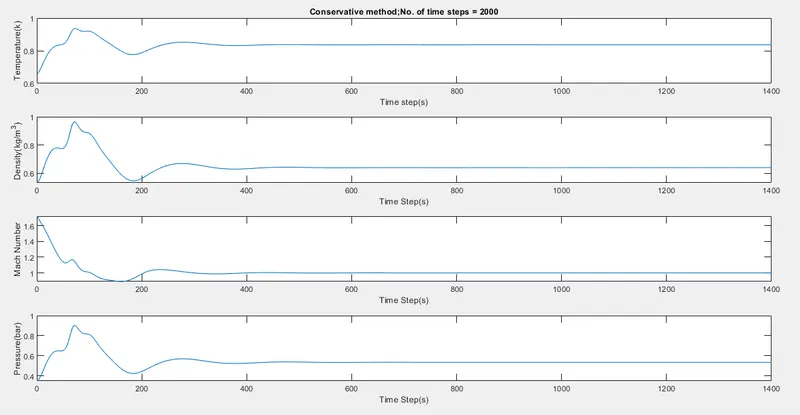
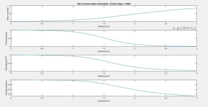
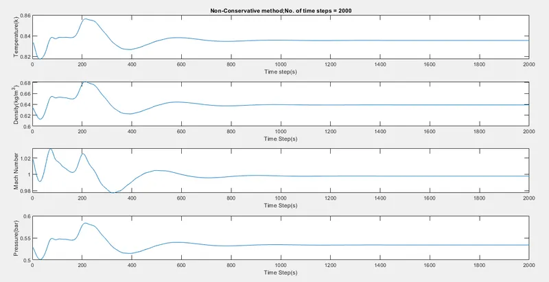
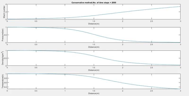
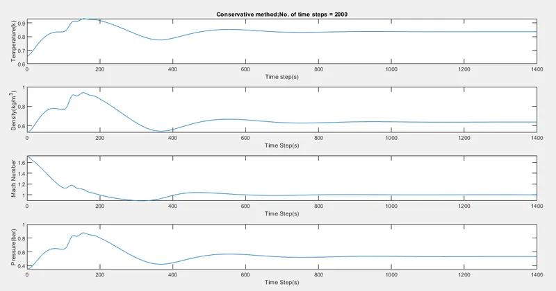
• The graphs are showing the steady-state distribution of density, velocity, temperature, and pressure along the nozzle length in x directions.
• Obtained graphs are in good agreement with the analytical solution.Both conservative and non-conservative, there is no variation in density and pressure.
• Value of velocity at the outlet is slightly high in conservative form solution than non-conservative form solution
• The value of temperature at the outlet is almost zero in conservative form solution and non-zero in non-conservative form solution(but variations are negligible)..
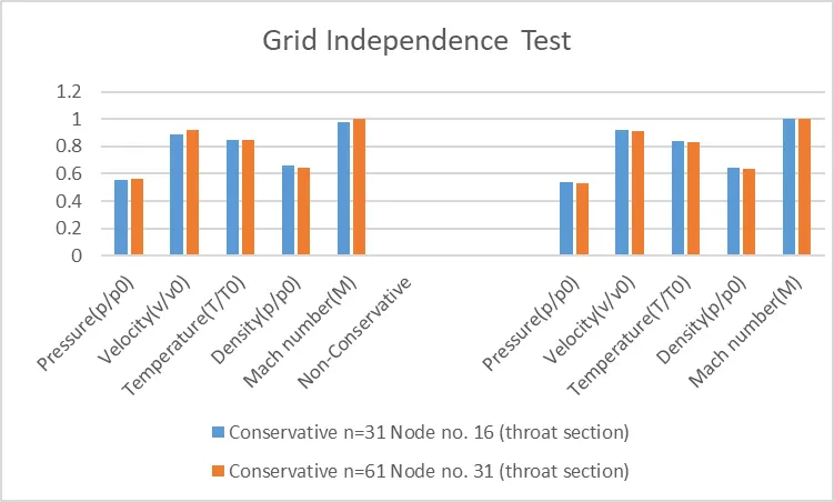
• Grid wise also, there is very negligible fluctuation in the flow variables value

When comparing mass flow rate, non-conservative solution seems to be more closer to the analytical solution

Fom the results it is clear that non-conservative method is taking more time than conservative method for convergence.

Grid independence test

Conservative
	n=31	n=61
	Node no. 16 (throat section)	Node no. 31 (throat section)
Pressure(p/p0)	0.553	0.561
Velocity(v/v0)	0.891	0.918
Temperature(T/T0)	0.849	0.846
Density(p/p0)	0.6631	0.641
Mach number(M)	0.977	0.9982
Non-Conservative
	n=31	n=61
	Node no. 16 (throat section)	Node no. 31 (throat section)
0Pressure(p/p0)	0.539	0.5327
Velocity(v/v0)	0.921	0.9138
Temperature(T/T0)	0.841	0.8345
Density(p/p0)	0.64	0.6381
Mach number(M)	0.999	0.9995

From the results we can observe that ,

As the number of grid points increases, the steady-state numerical results approach analytical value.
We may evaluate the following a from both conservative and non-conservative perspectives.
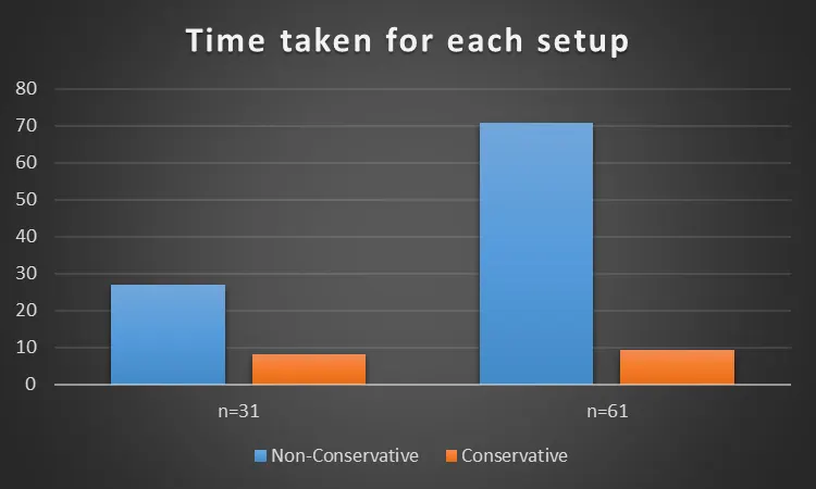
Conservation form results in a superior mass flow distribution or mass conservation. This may be seen in the mass flow rate vs time step graph or the mass flow rate vs. distance graph, where the results appear to be more consistent for the conservative form. The conservative form has less variance than the non-conservative form and tends to keep a consistent line.
The non-conservative form results in a lower residual. In the sense that residual decay is an indication of numerical algorithm quality, the non-conservative form performs better.
For primitive variables, the non-conservative form appears to yield somewhat more accurate findings, whereas the conservative form appears to produce slightly more accurate results for flux variables. In either situation, the outcomes are good.