Challenge

Week 3 - Solving second order ODEs

IIssac Alexander10 May 2022

In this program a Second Order ordinary differential equation is solved using Matlab software to obtain the solutions.

The ODE used in this program is an equation defining the motion of a simple pendulum when the initial conditions are provided.

The ODE is as follows

The terms in the ODE are

g = gravity in m/s2,

L = length of the pendulum in m,

m = mass of the ball in kg,

b=damping coefficient.

and theta which the pendulum makes to origin.

As we know in Matlab we can solve only first order ODEs, So using a function we are transforming second order ODE into first order.The function is as follows

function [dtheta_dt] = second_order_ode_solver(t,theta,b,g,l,m)

theta1=theta(1)

theta2=theta(2)

dtheta1_dt=theta2

dtheta2_dt= -b/m*dtheta1_dt -g/l*sin(theta1)

dtheta_dt=[dtheta1_dt; dtheta2_dt]

end

We have wrote second order in terms of first order terms such as theta2 & theta1.

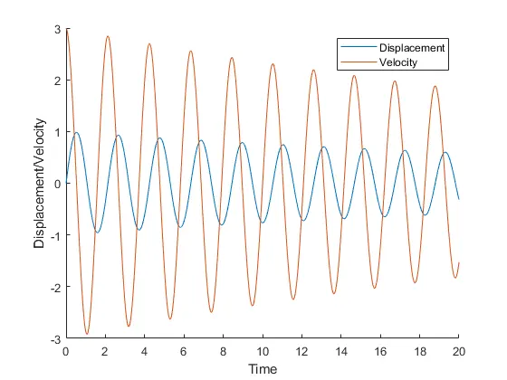
Also we are getting two outputs i.e Displacement(dtheta1/dt) & Velocity(dtheta2/dt)

Then coming to the main program, we need to provide all the intial conditions as specified in the question

L=1 metre,

m=1 kg,

b=0.05.

g=9.81 m/s2.

intial boundary conditions such as time=0 & velocity=3 rad/s

A time span of 20 second is also given

clear all

close all

clc

%inputs

l=1;

m=1;

g=9.81;

b=0.05;

%initial conditions

theta_0=[0;3]

%timespan of oscillation

t_span = linspace(0,20,500);

%solving the ODE

[t,results]=ode45(@(t,theta)second_order_ode_solver(t,theta,b,g,l,m),t_span,theta_0)

displacement=results(:,1);

velocity=results(:,2);

figure(1)

hold on

plot(t_span,displacement)

plot(t_span,velocity)

xlabel('Time')

ylabel('Displacement/Velocity')

legend('Displacement','Velocity')

hold off

%creating animation

%first defining start and endpoint of pendulum leg

ct=1;

for i = 1:length(t)

x0=0;

y0=0;

x1=-l*sin(results(:,1))

y1=-l*cos(results(:,1))

figure(2)

plot([x0 x1(i)],[y0 y1(i)],LineWidth=2)

hold on

plot(x1(i),y1(i),'o','MarkerSize',25,'MarkerFaceColor','r','MarkerEdgeColor','b')

xlabel('x-axis')

ylabel('y-axis')

axis([-1 1 -1.5 1])

grid on

hold off

M(ct)=getframe(gcf);

ct=ct+1

end

movie(M)

Pendulum_Oscillation = VideoWriter('Simple_Pendulum_Oscillation.avi')

open(Pendulum_Oscillation)

writeVideo(Pendulum_Oscillation,M)

close(Pendulum_Oscillation)

Command Usage

Linspace command is used to divide time between 0 to 20 sec into 500 equal steps.

Built-in ODE solver 'ode45' is used to solve the ODE & given the inputs as per the specified order.

Hold on & off command are used to incorporate two plots in one figure window.

xlabel and ylabel is used to given x&y axis names.

Using forloop the different positions of pendulum at different time steps are captured as image.

Using ct for each iteration using VideoWriter & writeVideo commands the animation is generated.

The MarkerSize,MarkerFaceColor,MarkerEdgeColor are used to define the size & color of bob at the end of pendulum

Errors Occured

After using hold on inside the for loop,not using hold off at the end resulted in n number of pendulum images in figure(2)

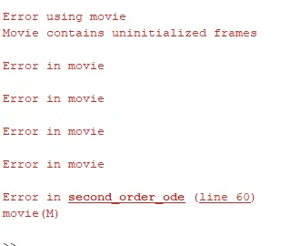
Adding ct=ct+1 before M(ct)=getframe(gcf); resulted in error.

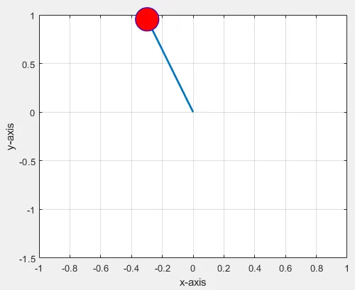
Fixing pendulum on origin(0,0) and using positive values for x1 & y1 resulted in an inverted pendulum plot.

Results obtained after rectifying the errors are

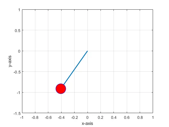
The link for the youtube video is https://youtu.be/7X_0wbALue4

Thank you

Week 3 - Solving second order ODEs

Ship work like this
in your own course.

Talk to a career counsellor

Ship work like thisin your own course.

Talk to a career counsellor

Ship work like this
in your own course.