Week 7 - Simulation of a 1D Super-sonic nozzle flow simulation using Macormack Method
Aim
1. To derive the conservation and non conservation form for the subsonic supersonic flow nozzle through the nozzle using Mac-cormack's technique.
2.To simulate the subsonic supersonic flow nozzle through the nozzle using Mac-cormacks technique(for both conservation and non conservation form
3.To determine the steady-state temperature distribution of flow field variables.
4. To study the difference between the conservative and non-conservative form of governing equations.
Introduction:
In the flow consideration, the nozzle is a convergent-divergent nozzle where the convergent part of the nozzle is attached to the reservoir which has stagnant pressure and temperature. The flow through the nozzle is isentropic flow. The area of the convergent nozzle is large hence the initial velocity is low and at the throat of the nozzle, the flow is sonic where Mach number(M) =1 and with increasing the area the velocity increases at this stage the flow breaks the sound barrier and attains supersonic speed where Mach number>1.
Mac Cormack's Method:
In CFD, MacCormack's technique is widely used in the discretization scheme for parabolic partial differential equations. The PDE is of second order.The MacCormack technique proceeds in two steps i.e., the predictor step followed by the corrector step.In the predictor step, the gradient value of the governing equation at time step n is estimated with known values at time step n. In this step forward differencing scheme is used.Then flow variables are calculated at time step n+1 with known values of flow variable at time step n along with gradient.In the corrector step, the values of the gradient at time step n+1 is estimated with the known values at time step n+1 i .e. obtained from the predicted step. In this step backward differencing scheme is used.The average of the gradients of the predicted step and corrector step is calculated.Then flow variables at the n+1 time step are calculated using flow variables at time step n and average gradients are calculated.
Governing Equations for conservative form
Continuity Equation
`(del(rho A))/(delt)+(del(rhoAV))/(delx)=0`
Momentum Equation
`(del(rho'A'V'))/(delt')+(del(rho'A'V'^(2)+(1/gamma)rho'A'))/(delx')`=`1/gammap'(delA)/(delx)`
Energy equation
`(del(rho'((e')/(gamma-1)+gamma/2V'^(2))A'))/(delt')`+`(del(rho'((e')/(gamma-1)+gamma/2V'^(2))V'A'+rho'A'V'))/(delx')=0`
Governing Equations for nonconservative form
Continuity Equation
`(delrho')/(delt')=-rho'(delV')/(delx')-rho'V'(del(lnA'))/(delx')`-`V'(delrho')/(delx')`
Momentum equation
`(delV')/(delt')=-V'(delV')/(delx')-1/(gamma)((delT')/(delx')`+`(T')/(rho')(delrho')/(delx'))`
Energy equation
``(delT')/(delt')=-V'(delT')/(delx')-(gamma-1)T'((delV')/(delx')``+`V'(del(lnA'))/(delx'))`
In the above equation (') on the flow variables represent that they are non-dimensionalized.
V' =Velocity
T' = Temperature
ρ'= Density
A'= Area of nozzle
t'=Time
gamma=Specific heat ratio=1.4
Discretization of equations :
We have finally set up that particular form of the equations that will be most appropriate as well as convenient for the time-marching solution of quasi-one-dimensional nozzle flow. This method is a simplified form of solving PDE's, as second-order degree equations are hard to solve,by the use of this method we get second-order accurate time marching without much effort .So Macormack method is an easy form of explicit finite-difference technique which is second-order-accurate in both space and time .It consists of two steps predictor and corrector.
First, consider the predictor step,In this step, we set up the spatial derivatives as forward differences. Also, to reduce the complexity of the notation, we will drop the use of the prime to denote a dimensionless variable. In what follows, all variables are the nondimensional variables, denoted earlier by the prime notation.As it is a explicit method ,we find the time derivative terms by using the previous state values and update the flow field variables.Then we proceed with corrector step. We then calculate the time derivatives by using these updated values by using backward difference. Then the average value of these time derivatives is found out.
`((delrho)/(delt))_(av)=0.5[((delrho)/(delt))_i^(t)+((delrho)/(delt))_i^(t+dt)]`
`((delV)/(delt))_(av)`=`0.5[((delV)/(delt))_i^(t)+((delV)/(delt))_i^(t+dt)]`
`((delT)/(delt))_(av)=0.5[((delT)/(delt))_i^(t)+((delT)/(delt))_i^(t+dt)]`
By using this average value we find the corrected values of flow field variables at time t+dt.These steps should be repeated until steady state is reached.
`rho_i^(t+dt)=rho_i^(t)+((delrho)/(delt))_(av)dt`
`V_i^(t+dt)=V_i^(t)+((delV)/(delt))_(av)dt`
`T_i^(t+dt)=T_i^(t)+((delT)/(delt))_(av)dt`
Calculation of time step (dt) :
`dt=C(dx/(sqrtT+V))`
Calculate dt at all the grid points, i = 1 to i = 31, by taking C =0.5, and then choose the minimum value among them.The resulting Δt obtained is used in the above equations to calculate flow field variables.
Nozzle Shape and Initial Conditions :
The nozzle shape, A = A(x), is specified and held fixed, independent of time, For the case illustrated in this section, we choose a parabolic area distribution given by
`A=1+2.2(x-1.5)^(2)` `0<=x<=3`
Therefore, in our choice of initial conditions, we have use any knowledge we may have about a given problem in order to intelligently pick some initial conditions so that they are choosen close to steady state values so that there will be no chance of solution to go unstable. For example, in the present problem, we know that density and T decrease and V increases as the flow expands through the nozzle. Hence, we choose initial conditions that qualitatively behave in the same fashion. For simplicity, let us assume linear variations of the flow-field variables, as a function of x. For the present case, we assume the following values at time t = 0.
initial conditions at t=0
`rho=1-0.3146x`
`T=1-0.2314x`
`V=(0.1+1.09x)T^(1/2)`
Boundary conditions :
Another aspect of the numerical solution is that of boundary conditions-an all-important aspect, because without the physically proper implementation of boundary conditions and their numerically proper representation, we have no hope whatsoever in obtaining a proper numerical solution to our flow problem.
Subsonic inflow boundary (point 1) :
Here, we must allow one variable to float.We choose the velocity V1, because on a physical basis we know the mass flow through the nozzle must be allowed to adjust to the proper steady state, and allowing V1 to float makes the most sense as part of this adjustment. The value of V1 changes with time and is calculated from information provided by the flow-field solution over the internal points. We use linear extrapolation from points 2 and 3 to calculate V1 and we take rho(1) =1 and T(1) =1 as fixed values.
`V_1=2V_2-V_3`
Supersonic outflow boundary (point N) :
Here, we must allow all flow-field variables to float We again choose to use linear extrapolation based on the flowfield values at the internal points. Specifically, we have, for the nondimensional variables,
`V_N=2V_N-1-V_N-2`
`rho_N=2rho_N-1-rho_(N-2)`
`T_N=2T_(N-1)-T_(N-2)`
Now we write a program using this data and do simulation to find out the flow field variables and required data.
Again writing conservation forms of mass,momentum and energy equations to apply MacCormacks method
Continuity Equation
`(del(rho A))/(delt)+(del(rhoAV))/(delx)=0`
Momentum Equation
`(del(rho'A'V'))/(delt')+(del(rho'A'V'^(2)+(1/gamma)rho'A'))/(delx')`=`1/gammap'(delA)/(delx)`
Energy equation
`(del(rho'((e')/(gamma-1)+gamma/2V'^(2))A'))/(delt')`+`(del(rho'((e')/(gamma-1)+gamma/2V'^(2))V'A'+rho'A'V'))/(delx')=0`
Let us express the equations for quasi-onedimensional flow in generic form. Let us define the elements of the solutions vector U, the flux vector F, and the source term J as follows.
`U_1=rho'A'`
`U_2=rho'A'V'`
`U_3=rho'((e')/(gamma-1)+gamma/2V'^(2))A'`
`F_1=rho'A'V'`
`F_2=rho'A'V'^(2)+1/gammaP'A'`
`F_3=rho'((e')/(gamma-1)+gamma/2V'^(2))V'A'+P'A'V'`
`J_2=1/gammaP'(delA')/(delx')`
Now substituting these terms in the above governing equations we get,
`(delU1)/(delt')=-(delF1)/(delx')`
`(delU_2)/(delt')=(delF_2)/(delx')+J_2`
`(delU_3)/(delt')=-(delF_3)/(delx')`
To obtain the primitive variables (V, T,P`rho`, etc.), we must decode the elements U1, U2, and U3 as follows. From the definitions of U1 , U2 , and U3 given above, we have
`rho'=(U_1)/(A')`
`V'=U_2/U_1`
`P'=rho'T'`
`e'=T'`
In the above equations, we note that the flux vector elements F1, F2, and F3 and source terms are couched in terms of the primitive variables. When the computer program is written with F 1 , F2 , and F3 expressed directly in terms of `rho'`, V', P', and e', instabilities develop during the course of the time-marching solution .So,we write such that the governing equations are in Pure form in terms of the elements of the solution vector i.e, in terms of U1,U2 and U3.
`F_1=U_2`
`F_2=U_2^(2)/U_1+(gamma-1)/(gamma)(U_3-gamma/2U_2^(2)/U_1)`
`F_3=(gamma(U_2U_3)/U_1-(gamma(gamma-1))/(2)U_2^(3)/U_1^(2))`
`J_2=1/gammarho'T'(delA')/(delx')`
Finally the next step to do is discretization .We take the governing equations that consists of flux terms and source terms and discretize them by using MacCormack's method.
Predictor step:. To start the calculation, we use the initial conditions for U1, U2, and U3 to calculate the initial values of F1, F2, and F3 and and we use these values to calculate the values of U1,U2 and U3 in the next time step .Calculating the time derivatives by using forward difference to the RHS terms to discretize and these time derivatives are used to calculate the predicted values of U1 ,U2 and U3.
Corrector Step : Now using the predicted values we calculate the new flux terms and source terms .Then we calculate the time derivative terms by using backward difference.Then we calculate the average values of time derivatives of predictor and corrector steps .
`((delU_1)/(delt))_(av)=0.5[((delU_1)/(delt'))_(i)^(t')+``((delU_2)/(delt'))_i^(t'+trianglet')]`
`((delU_2)/(delt))_(av)=0.5[((delU_2)/(delt'))_(i)^(t')`+`((delU_2)/(delt'))_i^(t'+trianglet')]`
``((delU_3)/(delt))_(av)=0.5[((delU_3)/(delt'))_i^(t')+((delU_3)/(delt'))_i^(t+trianglet)]`
Then we calculate the corrected values of U1,U2,U3 by using average values of time derivative.This is done at every node except the boundary nodes since we calculate them by using boundary conditions.Then we also calculate primitive variables.These steps are to be repeated until steady state is obtained.
`(U_1)_i^(t'+trianglet')=(U_1)_i^(t')+((delU1)/(delt'))_(av)(trianglet)`
`(U_2)_i^(t'+trianglet')=(U_2)_i^(t')+((delU2)/(delt'))_(av)(trianglet)`
`(U_3)_i^(t'+trianglet')=(U_3)_i^(t')+((delU_3)/(delt'))_(av)trianglet`
Initial conditions :
The nozzle shape, A = A(x), is specified and held fixed, independent of time, For the case illustrated in this section, we choose a parabolic area distribution given by

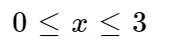
Since the dependent variables being solved in governing are U1, U2, and U3, we need initial conditions for these same variables at time t = 0 in order to start the finite-difference solution. The initial conditions for U1, U2, and U3 also allow initial conditions for F1 F2 and F3 to be obtained from above equations. Such initial conditions for F1, F2, and F3 are needed to form the x derivatives on the right-hand sides of the governing equations at the first time step.
The initial conditions for U1 , U2, and U3 were synthesized by assuming the following variations for ρ' and T':
`rho'=1,` T'=1 for `0<=x'<=0.5`
`rho'=1-0.366(x'-0.5),T'=1-0.167(x'-0.5)` for `0.5<=x'<=1.5`
`rho'=0.634-0.3879(x'-1.5),T'=0.833-0.3507(x'-1.5)` for `1.5<=x'<=3.5`
These variations slightly more realistic than those assumed in the Nozzle Shape and initial conditions for non conservative form this is in anticipation that the stability behaviour of the finite difference formulation using the conservation form of the governing equations might be slightly more sensitive, and therefore it is useful to start with more improve initial conditions than those given for non conservative form. The initial condition for the variation of V' is synthesized by taking advantage of the fact that one of the dependent variables in our governing equations, namely U2 is physically the local mass flow; that is, U2= ρ'A'V'. Therefore,for the initial conditions only, let us assume a constant mass flow through the nozzle and calculate V' as `V'=U_2/(rho'A')=0.59/(rho'A')`
The value 0.59 is chosen for U2 because it is close to the exact analytical value of the steady-state mass flow (which for this case is 0.579). Therefore, the initial condition for V' as a function of x' is obtained by substituting the p' variation given by above equations.Finally, the initial conditions for U1 , U2, U3 are obtained by substituting the above variations for p',
T', and V' into the definitions above
`U_1=rho'A'`
`U_2=rho'A'V'`
`U_3=rho'((e')/(gamma-1)+gamma/2V'^(2))A'`
Boundary conditions :
Subsonic inflow boundary (point 1) :
At the subsonic inflow boundary two properties are held fixed and one is allowed to float, and at the supersonic outflow boundary all properties are allowed to float. In the present formulation, as before, we hold `rho' and T' fixed at the inflow boundary, both equal to 1.0, and allow V' to float. By holding `rho'` fixed, then U1 at grid point i = 1 is fixed, independent of time, via `U_1=rho'A'` That is,
`(U_1)_(i=1)=(rho'A')_(i=1)=A_(i=1)^(')=`fixed value
`U_2(i=1)=2(U_(2))_(i=2)-(U_2)_(i=3)`
`U_3=rho'((e')/(gamma-1)+gamma/2V'^(2))A'`
Supersonic outflow boundary (point N) :
At the supersonic outflow boundary all properties are allowed to float.The flow properties at the downstream, supersonic outflow boundary are obtained by linear extrapolation from the two adjacent internal points. If N denotes the grid point at the outflow boundary, then
`(U_1)_N=2(U_1)_(N-1)-(U_1)_(N-2)`
`(U_2)_N=2(U_2)_(N-1)-(U_2)_(N-2)`
`(U_3)_N=2(U_3)_(N-1)-(U_3)_(N-2)`
MATLAB CODE MAIN PROGRAMME
clear all
close all
clc
%specifying grd points
n=31;  %41,51,61

x=linspace(0,3,n);
%calling functions for both non conservative and conservative forms
% [rho_nc,v_nc,T_nc,P_nc,Ma_nc,m_nc,rho_t_nc,v_t_nc,T_t_nc,P_t_nc,Ma_nc_t_nc]=nonconservative()
[rho,v,T,P,Ma_nc,m_nc,rho_t,v_t,T_t,P_t,Ma_nc_t]=nonconservative();
%[rho,v,T,P,Ma_c,m,rho_t,v_t,T_t,P_t,Ma_c_t]=conservative()
[rho,v,T,P,Ma_c,m_c,rho_t,v_t,T_t,P_t,Ma_c_t]=conservative()
figure(20)
plot(x,m_nc,DisplayName='Non Conservative')
hold on
plot(x,m_c,DisplayName='Conservative')
title('comparison of mass flow rates of conservative and non conservative')
xlabel('length of nozzle')
ylabel('nondimension mass flow rate')
legend('Non conservative form','Conservative form')
%%%%%%%%%%%%%%%%%%%%%%%%%%%%%%%%%%%%%%
Explanation of main programme
1. Defining the number of grid points.
2. Calling the functions of both non-conservable and conservable forms
3. Plotting of the graph which compares the mass flow rate of conservative and non-conservative form.
%%%%%%%%%%%%%%%%%%%%%%%%%%%%%%%%%%%%%%%%%%%%
Function to calculate the flow variables of the non-conservative form of subsonic supersonic flow through a nozzle.
function[rho,v,T,P,Ma_nc,m_nc,rho_t,v_t,T_t,P_t,Ma_nc_t]=nonconservative()
%inputs
n=31;
x=linspace(0,3,n);
dx=x(2)-x(1);

%calculate initial profile
rho= 1-0.3146*x;
T= 1-0.2314*x;
v= (0.1+1.09*x).*T.^0.5;

gamma=1.4;
% area
a=1+2.2*(x-1.5).^2;
%time steps
nt=1400;
cfl=0.5;
dt=min((cfl*dx)./(v+sqrt(T)));
throat=find(a==1);
Ma_nc=v./sqrt(T);


%outer loop
for k=1:nt
    dt=min((cfl*dx)./(v+sqrt(T)));
    rho_old=rho;
    T_old=T;
    v_old=v;


    % predictor method
    for j=2:n-1
        dvdx=(v(j+1)-v(j))/dx;
        drhodx=(rho(j+1)-rho(j))/dx;
        dTdx=(T(j+1)-T(j))/dx;
        dlogadx=(log(a(j+1))-log(a(j)))/dx;

        %continuity equation
        drhodt_p(j)=-rho(j)*dvdx-rho(j)*v(j)*dlogadx-v(j)*drhodx;
        %momentum equation
        dvdt_p(j)=-v(j)*dvdx-(1/gamma)*(dTdx+(T(j)/rho(j))*drhodx);
        %energy equation
        dTdt_p(j)=-v(j)*dTdx-(gamma-1)*T(j)*(dvdx+v(j)*dlogadx);

        %Intermediate Solution Update
        v(j)=v(j)+dvdt_p(j)*dt;
        rho(j)=rho(j)+drhodt_p(j)*dt;
        T(j)=T(j)+dTdt_p(j)*dt;

    end

    %  corrector method
    for j=2:n-1
        dvdx=(v(j)-v(j-1))/dx;
        drhodx=(rho(j)-rho(j-1))/dx;
        dTdx=(T(j)-T(j-1))/dx;
        dlogadx=(log(a(j))-log(a(j-1)))/dx;

        %continuity equation
        drhodt_c(j)=-rho(j)*dvdx-rho(j)*v(j)*dlogadx-v(j)*drhodx;
        %momentum equation
        dvdt_c(j)=-v(j)*dvdx-(1/gamma)*(dTdx+(T(j)/rho(j))*drhodx);
        %energy equation
        dTdt_c(j)=-v(j)*dTdx-(gamma-1)*T(j)*(dvdx+v(j)*dlogadx);
    end

    %compute the average time derivative
     drhodt=0.5*(drhodt_p+drhodt_c);
     dvdt=0.5*(dvdt_p+dvdt_c);
     dTdt=0.5*(dTdt_p+dTdt_c);


	%Final solution update
    for i=2:n-1
		rho(i)=rho_old(i)+drhodt(i)*dt;
		v(i)=v_old(i)+dvdt(i)*dt;
		T(i)=T_old(i)+dTdt(i)*dt;
    end
    % applying bc
    %inlet
    v(1)=2*v(2)-v(3);
    %outlet
    v(n)=2*v(n-1)-v(n-2);
    rho(n)=2*rho(n-1)-rho(n-2);
    T(n)=2*T(n-1)-T(n-2);

 %calculate the pressure,tempr,density,mach number at throat(area ratio=1)
   rho_t(k)=rho(throat);
   T_t(k)= T(throat);
   P_t(k)=rho(throat).*T(throat);
   v_t(k)=v(throat);
   Ma_nc_t(k)=v(throat)./sqrt(T(throat));

    m_nc=rho.*v.*a;
    figure (1)
    hold on
    if k==50
        plot(x,m_nc,DisplayName=['Time step = ',num2str(k)])
    end
    if k==100
        plot(x,m_nc,DisplayName=['Time step = ',num2str(k)])
    end
    if k==200
        plot(x,m_nc,DisplayName=['Time step = ',num2str(k)])
    end
    if k==700
        plot(x,m_nc,DisplayName=['Time step = ',num2str(k)])
    end
% add the rest here

    figure (1)
    legend
    xlabel('Length of the nozzle')
    ylabel('Mass flow rate')

end
  %Calculating pressure and mass flow rate
   P=rho.*T;
   m_nc=rho.*v.*a;
    figure(2)
    subplot(4,1,1)
    plot(x,Ma_nc,'r',LineWidth=1)
    xlabel('Length of nozzle')
    ylabel('Mach number')


    subplot(4,1,2)
    plot(x,T,'b',LineWidth=1)
    xlabel('Length of nozzle')
    ylabel('Temperature')


    subplot(4,1,3)
    plot(x,rho,'y',LineWidth=1)
    xlabel('Length of nozzle')
    ylabel('density')

    subplot(4,1,4)
    plot(x,P,'g',LineWidth=1)
    xlabel('Length of nozzle')
    ylabel('pressure')

 figure(3)
    subplot(4,1,1)
    plot(Ma_nc_t,'r',LineWidth=1)
    xlabel('Time Step')
    ylabel('Mach number')


    subplot(4,1,2)
    plot(T_t,'b',LineWidth=1)
    xlabel('Time Step')
    ylabel('Temperature')


    subplot(4,1,3)
    plot(rho_t,'y',LineWidth=1)
    xlabel('Time Step')
    ylabel('density')

    subplot(4,1,4)
    plot(P_t,'g',LineWidth=1)
    xlabel('Time Step')
    ylabel('pressure')

end
Explanation of the above function used for non-conservation form:
1. Function takes the number of grid points(n) as input.
2. With n, the position of the grid points is obtained and grid spacing is calculated.
3. With the position of the grid points are known the initial boundary conditions for the flow variables are calculated.
4. Heat capacity ratio is defined and throat position is found using find command with condition a==1.
5. The governing equation of non-conservative form is of explicit form which is governed by stability criteria where CFL =0.5 with which the time step size is calculated.
6. Time loop is created to calculate the steady-state flow variables. No. of the time loop is of 1400.
7. Inside the time loop, a copy of the previous iteration time step value is made which is later used in the final update of the solution.
8. For the calculation of the predicted values for each time step a for loop is created. The for loop is between the 2nd grid point to the 30th grid point since the initial and last boundary values are defined in boundary conditions.
Flow variables are updated using the predicted step derived above for non-conservative form inside the predictor for loop.
9. Another for loop is created to calculate the gradients for the corrector step using the equation derived for non-conservative form.
10. Then the average of the predictor and corrector gradients are calculated.
11. Another for loop is created for the final update of the flow variables with the gradient average.
12. Inflow and outflow boundary conditions are defined. The reason for defining them at the end of the calculation is that the value of the boundaries depends on the converged values of the inner grid points. Hence the boundary conditions for the flow variables are defined at the end.
13. Storing the values of the flow variables at the throat section to plot the time-wise variation of the flow variables at the throat.
14. If end statements are created to plot the mass flow rate at different time steps to study the variation of the mass flow rate at different time steps till it reaches the steady-state.
15. Mach number(Ma_nc), pressure(P_nc) and mass flow rate(m_nc) is calculated.
16. Two plots are created one for steady-state distribution of the flow variables for the length of the nozzle and time-wise variation of the flow variables for the number of time steps.
%%%%%%%%%%%%%%%%%%%%%%%%%%%%%%%%%%%%%%%%%%%%%
Function to calculate the flow variables of the conservative form of subsonic supersonic flow through a nozzle.
function[rho,v,T,P,Ma_c,m_c,rho_t,v_t,T_t,P_t,Ma_c_t]=conservative()
x = linspace(0,3,31);
n = 31;

dx = x(2)-x(1);

for i= 1:length(x)
    if x(i)>=0 && x(i)<=0.5
        rho(i) = 1;
        T(i)= 1;
    elseif x(i)>=0.5 && x(i)<=1.5
        rho(i) = 1.0-0.366*(x(i)-0.5);
        T(i) =   1.0-0.167*(x(i)-0.5);
    elseif x(i)>=1.5 && x(i)<=3.5
        rho(i) = 0.634-0.3879*(x(i)-1.5);
        T(i) = 0.833-0.3507*(x(i)-1.5);
    end
end

a = 1+2.2*(x-1.5).^2;
v = 0.59./(rho.*a);
cfl = 0.5;
gamma = 1.4;
throat=find(a==1);

u1= rho.*a;
u2= rho.*a.*v;
u3= rho.*a.*((T./(gamma-1))+(gamma/2).*v.^2);
nt = 1400;
%dt = 0.01;
for z= 1:31
    u = (T(z))^(1/2);
    dt(z)= cfl*dx/(u+v(z));
end
dt=min(dt);


%figure(1)
%plot(x, u1, x, u2, x, u3)


for k =1:nt
    % storing initial terms
    u1old = u1;
    u2old =u2;
    u3old =u3;
    % calculating flux terms

    F1= u2;
    F2= ((u2.^2)./u1 )+ ((gamma-1)/gamma)*(u3-((gamma/2) * (u2.^2)./u1));
    F3= ((gamma*u2.*u3)./u1) - ((gamma*(gamma-1)/2) * (u2.^3)./(u1.^2));

    % predictor method
    for j= 2:n-1
        % calculating source term
        J2(j) =   (1/gamma)*rho(j)*T(j)*((a(j+1)-a(j))/dx);
        du1dt_p(j) = -(F1(j+1)-F1(j))/dx;
        du2dt_p(j) = -(F2(j+1)-F2(j))/dx + J2(j);
        du3dt_p(j) = -(F3(j+1)-F3(j))/dx;

        % updating new values
        u1(j) = u1(j)+du1dt_p(j).*dt;
        u2(j) = u2(j)+du2dt_p(j).*dt;
        u3(j) = u3(j)+du3dt_p(j).*dt;

    end

    % updated values
    rho = u1./a;
    v= u2./u1;
    T= (gamma-1)*(u3./u1-(gamma/2)*v.^2);
    %updating flux values

    F1= u2;
    F2= ((u2.^2)./u1 )+ ((gamma-1)/gamma)*(u3-((gamma/2) * (u2.^2)./u1));
    F3= ((gamma.*u2.*u3)./u1) - ((gamma*(gamma-1)/2) * (u2.^3)./(u1.^2));

    % corrector method
    for j= 2:n-1
        %updating source term
        J2(j) = (1/gamma)*rho(j)*T(j)*((a(j)-a(j-1))/dx);
        du1dt_c(j) = -(F1(j)-F1(j-1))/dx;
        du2dt_c(j) = -(F2(j)-F2(j-1))/dx + J2(j);
        du3dt_c(j)= -(F3(j)-F3(j-1))/dx;
    end

    % calculating avg
    du1dt_avg = 0.5.*(du1dt_p +du1dt_c);
    du2dt_avg = 0.5.*(du2dt_p +du2dt_c);
    du3dt_avg = 0.5.*(du3dt_p +du3dt_c);

%
    for w = 2:n-1
        u1(w) = u1old(w) + du1dt_avg(w)*dt;
        u2(w) = u2old(w) + du2dt_avg(w)*dt;
        u3(w) = u3old(w) + du3dt_avg(w)*dt;
    end

    %boundary conditions
    u1(1) = rho(1).*a(1);
    u2(1)= 2*u2(2)-u2(3);
    u3(1)= u1(1)*((T(1)/(gamma-1))+(gamma/2)*v(1).^2);

    u1(n)= 2*u1(n-1)- u1(n-2);
    u2(n)= 2*u2(n-1)- u2(n-2);
    u3(n)= 2*u3(n-1)- u3(n-2);
    % calcultaing primitive variables
    rho = u1./a;
    v= u2./u1;
    T = (gamma-1)*((u3./u1)-(gamma/2)*v.^2);

    P= rho.*T;
    Ma_c = v./sqrt(T);


    %calculate the pressure,tempr,density,mach number at throat(area ratio=1)
   rho_t(k)=rho(throat);
   T_t(k)= T(throat);
   P_t(k)=rho(throat).*T(throat);
   v_t(k)=v(throat);
   Ma_c_t(k)=v(throat)./sqrt(T(throat));

    m_c=rho.*v.*a;
    figure (10)
    hold on
    if k==50
        plot(x,m_c,DisplayName=['Time step = ',num2str(k)])
    end
    if k==100
        plot(x,m_c,DisplayName=['Time step = ',num2str(k)])
    end
    if k==200
        plot(x,m_c,DisplayName=['Time step = ',num2str(k)])
    end
    if k==700
        plot(x,m_c,DisplayName=['Time step = ',num2str(k)])
    end
% add the rest here

    figure (10)
    legend
    xlabel('Length of the nozzle')
    ylabel('Mass flow rate')

end
  %Calculating pressure and mass flow rate
%    P=rho.*T;
%    m=rho.*v.*a;
 figure(11)
    subplot(4,1,1)
    plot(Ma_c_t,'r',LineWidth=1)
    xlabel('Time Step')
    ylabel('Mach number')


    subplot(4,1,2)
    plot(T_t,'b',LineWidth=1)
    xlabel('Time Step')
    ylabel('Temperature')


    subplot(4,1,3)
    plot(rho_t,'y',LineWidth=1)
    xlabel('Time Step')
    ylabel('density')

    subplot(4,1,4)
    plot(P_t,'g',LineWidth=1)
    xlabel('Time Step')
    ylabel('pressure')


 figure(12)
    subplot(4,1,1)
    plot(x,Ma_c,'r',LineWidth=1)
    xlabel('Length of nozzle')
    ylabel('Mach number')

    subplot(4,1,2)
    plot(x,T,'b',LineWidth=1)
    xlabel('Length of nozzle')
    ylabel('Temperature')

    subplot(4,1,3)
    plot(x,rho,'y',LineWidth=1)
    xlabel('Length of nozzle')
    ylabel('density')

    subplot(4,1,4)
    plot(x,P,'g',LineWidth=1)
    xlabel('Length of nozzle')
    ylabel('pressure')

end
Explanation of the above function used for conservation form:
1. Function takes the number of grid points(n) as input.
2. With n, the position of the grid points is obtained and grid spacing is calculated.
3. For loop is created for defining the initial boundary conditions with the equations specified in the introduction for conservative form
4. Since the flow variables are specified in terms of solution variables, the initial boundary conditions are defined for the solution variables and the position of the throat section is also found.
5. The governing equation of non-conservative form is of explicit form which is governed by stability criteria where CFL =0.5 with which the time step size is calculated.
6. Time loop is created to calculate the steady-state flow variables. No. of time loop is of 1400.
7. Inside the time loop, a copy of the previous iteration time step value is made which is later used in the final update of the solution.
8. Flux variables are calculated with solutions variables from each time step.
9. For loop is created in order to calculate the source term. For loop is created because the formula contains the difference term for the area and hence area form 1x30 matrix whereas the density and temperature are 1x31 matrices hence for loop is created which runs for 30 generating 1x30 matrix for j2.
10. For the calculation of the predicted values for each time step a for loop is created. The for loop is between the 2nd grid point to the 30th grid point since the initial and last boundary values are defined in boundary conditions.
Solution variables are updated using the predicted step derived above for the conservative form inside the predictor step for loop.
11. With the predicted solution variable density and temperature and flux variables are calculated.
12. Another for loop is created to calculate the gradients for the corrector step using the equation derived for conservative form with predicted flux variable.
13. Then the average of the predictor and corrector gradients are calculated.
14. Another For loop is created for the final update of the solution variables with the gradient average.
15. Inflow and outflow boundary conditions are defined. The reason for defining them at the end of the calculation is that the value of the boundaries depends on the converged values of the inner grid points. Hence the boundary conditions for the solution variables are defined at the end.
16. Flow variables are found from the converged solution variables for that time step in order to store the flow variables at the throat section for each time loop.
17. If end statements are created to plot the mass flow rate at different time steps to study the variation of the mass flow rate at different time steps till it reaches the steady-state.
18. Final flow variables are calculated at 1400 time steps at the end of the loop.
19. Plot is created for the steady-state and time-wise distribution of the converged flow variables.
%%%%%%%%%%%%%%%%%%%%%%%%%%%%%%%%%%%%%%%%%%%%%%
Results of graphs for both conservative and non-conservative forms
Nonconservation-form
.........................................................................................................................................
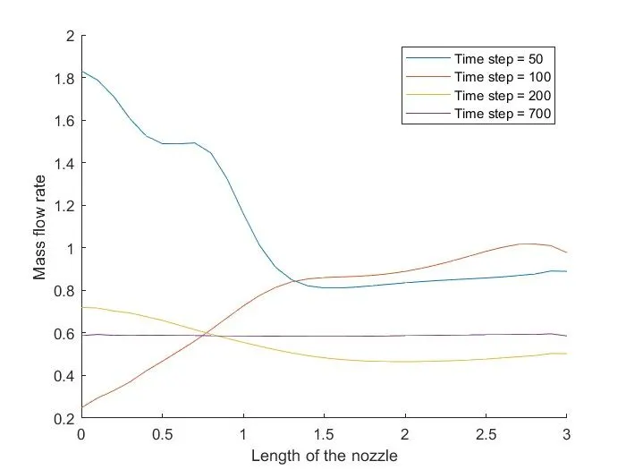
Mass flow rate at various time steps
........................................................................................................................................
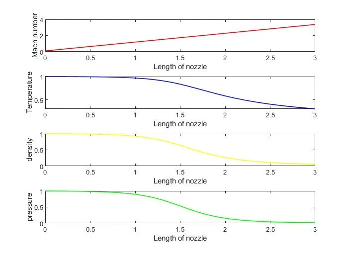
Steady-state distribution of primitive variables with respect to the length of the nozzle.
......................................................................................................................................
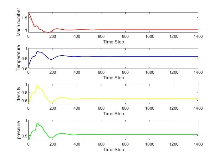
Time-wise distribution of flow variables at different time steps
......................................................................................................................................... For conservative form
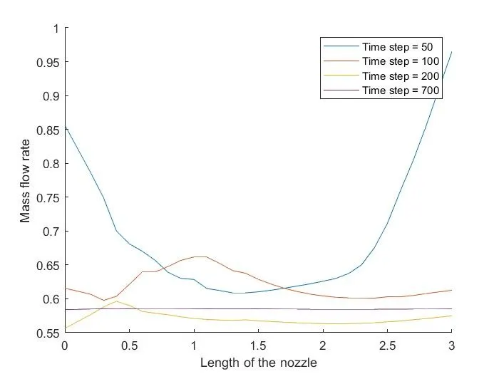
Mass flow rate at various time steps for conservative
.........................................................................................................................................
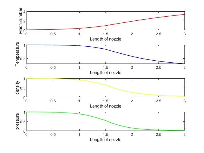
Steady-state distribution of primitive variables with respect to the length of the nozzle for conservative
.........................................................................................................................................
Time-wise distribution of flow variables at different time steps for conservative 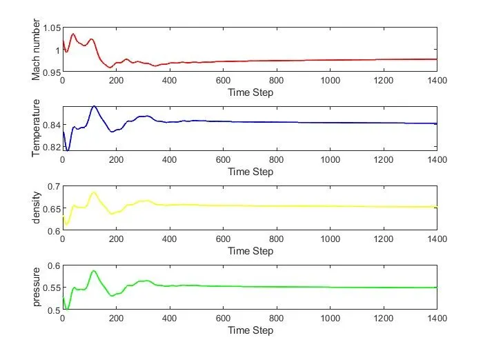
......................................................................................................................................
Grid inpendence Test:We did grid independence test for property density(non dimensional) for various gridpoints like n=15,31,63,121we are obtaining density values NA,0.6498,0.6377,0.6373.So from this result we will take 63 points as ptimum grid point,because after that the value become constant.
Explanation of the Output graph:
The flow variables density, temperature, and pressure decrease along the length of the nozzle whereas velocity and Mach number increases along the length of the nozzle, this type of behavior of the flow are because in the converging part of the nozzle the Mach number is less than 1 as it approaches throat, the area of the nozzle decreases and at the throat, the Mach number is equal to 1. The flow expands isentropically, as a result, the flow accelerates in the divergent part of the nozzle also due to an increase in area and decrease in pressure which results in a decrease in density.
Variations in flow variables are high at the initial time steps because the time derivatives are large and oscillate. The oscillations are due to unsteady compression and expansion of waves which propagate through the nozzle. As the time steps increase the flow reaches a steady-state the time derivatives become small and change in the order of six in their magnitude at larger time steps. As the flow attains the steady-state the time derivative becomes zero but when numerically solved this is not achieved. These non zero values are called residuals which are used by CFD experts in comparing the time marching solution of the steady-state with their magnitude and the rate of decay.
The same effect can be used to explain the non-dimensional mass flow rate at initial times there are large oscillations of mass flow rate along the length of the nozzle as the flow approaches steady state the mass flow rate is constant which can be seen at a 700th-time step it approaches the steady-state value 0.58 which is close to analytical value.
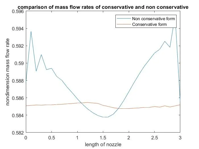
In the comparison of the mass flow rate between conservation and non-conservation form plot, we can infer that the mass flow rate is closer to the analytical solution. With this, we can say that the conservation form of the governing equations performs well in conserving the mass flow rate than the non-conservation form this is because in the conservation form the mass flow rate is one of the dependent variables whereas in the non-conservation form mass flow rate is calculated from the dependent variables i.e., flow variables.
Results and conclusion
1. The conservation form yields a better mass distribution.The conservation form simply does a better job of conserving mass
2.The nonconservation form leads to small residuals.The amount by which residual decays is often used as an index of quality of numerical algorithim.In this sense the nonconservation form does a better job.
3.The non conservation form seem to produce slightly more accurate results for primitive variables and conservation form seems to produce slightly more accurate results for flux variables.The results in either case are satisfactory.
4.Computational effort needed for conservation form is more as the flow variables need to be calculated from the solution variables whereas in the non-conservation form the converged flow variables are calculated directly.