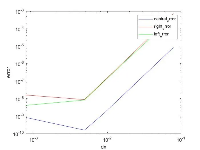
Week 3.5 - Deriving 4th order approximation of a 2nd order derivative using Taylor Table method
AIM : To derive the fourth order approximations of second order derivative by using central difference,skewed-right sided difference,skewed left sided difference and compare with numerical derivative of given function and plot graphs using MATLAB
Calculation of nodes for different schemes
For central difference the order of accuracy is P=N-Q+1
where P= order of accuracy
N=number of nodes
Q=order of derivative
4=N-2+1
N=5
Therefore we needed 5 nodes for fourth order approximations of second order derivative by using cen-tral difference.
`(del^(2)f)/(delx^(2))`=`af(i-2)+bf(i-1)+cf(i)+df(i+1)`+`ef(i+2)`....................................(1)
Let dx be the discretization size,then by taylor series expansion
`af(i-2)`=`a[f(i)-2dxf^(')(i)/1+4(dx)^(2)/2f''(i)``-8(dx)^(3)/6f'''(i)+16(dx)^(4)/24f^(4)(i)``-32(dx)^(5)/120f^(5)(i)+64(dx)^(6)/720f^(6)(i)]`
`bf(i-1)=b[f(i)-dx/1f'(i)+(dx)^(2)/2f^(2)(i)``-(dx)^(3)/6f^(3)(i)+(dx)^(4)/24f^(4)(i)-(dx)^(5)/120``+(dx)^(6)/720f^(6)(i)]`
`df(i+1)=b[f(i)+f'(i)(trianglex)+f''(i)``(trianglex)^(2)/2``+f^3(i)(trianglex)^(3)/6``+f^(4)(i)(trianglex)^(4)/24+f^(5)(trianglex)^(5)/120``+f^(6)(trianglex)^(6)/720]`
`ef(i+2)=e[f(i)+2dxf'(i)+4(dx)^(2)/2f^(2)(i)+8(dx)^(3)/6f^(3)(i)``+16(dx)^(4)/24f^(4)(i)+32/120(dx)^(5)f^(5)(i)+64/720(dx)^(6)f^(6)(i)]`
above expressions represented in tabular form
| f(i) | f'(i)dx | `f''(i)(dx)^(2)` | `f^(3)(i)(dx)^(3)` | `f^(4)(i)(dx)^(4)` | `f^(5)(i)(dx)^(5)` | `f^(6)(i)(dx)^(6)` | |
| `a.f(i-2)` | a | -2a | 2a | -8a/6 | 2a/3 | -4a/15 | 4a/15 |
| `b.f(i-1)` | b | -b | b/2 | -b/6 | b/24 | -b/120 | b/720 |
| `c.f(i)` | c | 0 | 0 | 0 | 0 | 0 | 0 |
| `d.f(i+1)` | d | d | d/2 | d/6 | d/24 | d/120 | d/720 |
| `e.f(i+2)` | e | 2e | 2e | 2e | 2e/3 | 4e/15 | 4e/45wi |
|
`(del^(2)f)/(delx^(2)`=sum of above rows in each column |
0 | 0 | 1 | 0 | 0 | will calculate | will calculate |
a+b+c+d+e=0
-2a-b+d+2e=0
2a+b/2+d/2+2e=1
-8a/6-b/6+d/6+8e/6+0
2a/3+b/24+d/24+2e/3=0
above equations representing in matrix form AX=B and solving
`[[1,1,1,1,1],[-2,-1,0,1,2],[2,1/2,0,1/2,2],[-8/6,-1/6,0,1/6,8/6],[2/3,1/24,0,1/24,2/3]]``[((a),(b),(c),(d),(e))]``=((0),(0),(1),(0),(0))`
solving the above matrix leads to a=-0.0833,b=1.3333,c=-2.5,d=1.3333,e=-0.0833,so finally we get a=e,b=d
because of that sum of coefficients of column 2=a+b+c+d+e=-0.0833+1.3333-2.5+1.3333-0.0833=0,similarly
sum of coefficients of third column=-2a-b+d+2e=-2a-b+b+2a=0
sum of coefficients of fourth column=2a+b/2+d/2+2e=2(-0.0833)+1.3333/2+1.3333/2+2(-0.0833)=1
sum of coefficients of fifth column=-8a/6-b/6+d/6+8e/6=0
sum of coefficients of sixth column=2a/3+b/24+d/24+2e/3=0(by subsituting values)
sum of coefficients of seventh column=0(because of a=e and b=d)
sum of coefficients of eight column=8a/45+b/360
Finally if you substituted in above equation (1) we wil get
`(del^(2)f)/(delx^(2))=`a.f(i-2)+b.f(i-1)+c.f(i)``+d.f(i+1)``+e.f(i+2)`=0+0+`f''(i)(dx)^(2)`+`((8a)/45+b/360)f^(6)(dx)^(6)`
`(del^(2)f)/(delx^(2))`=`[a.f(i-2)+b.f(i-1)+c.f(i)+d.f(i+1)+e.f(i+2)]/(dx)^(2)``+o(dx)^(4)`
SKEWED RIGHT-SIDED DIFFERENCES
For skewed scheme the order of accuracy is P=N-Q
where P= order of accuracy
N=number of nodes
Q=order of derivative
4=N-2
N=6
Therefore we needed 6 nodes for fourth order approximations of second order derivative by using skewed scheme
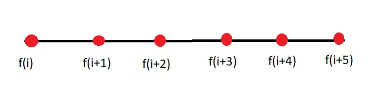
`(del^(2)f)/(delx^(2))`=`g.f(i)+h.f(i+1)+j.f(i+2)+k.f(i+3)+l.f(i+4)+m.f(i+5)`..........................(2`
Let dx be the discretization size
`h.f(i+1)=h[f(i)+dxf(i)'+(dx)^(2)/2f''(i)+(dx)^(3)/6.f^(3)(i)``+(dx)^(4)/24f^(4)(i)+(dx)^(5)/120f^(5)(i)+(dx)^(6)/720f^(6)(i)]`
`j.f(i+2)=i[f(i)+dxf'(i)+2dxf''(i)``+8/6(dx)^(3)f^(3)(i)+16(dx)^(4)/24f^(4)(i)``+32(dx)^(5)/120f^(5)(i)+64/720(dx)^(6)f^(6)(i)]`
`k.f(i+3)=j[f(i)+3dxf'(i)+9/4(dx)^(2)f''(i)``27/6(dx)^(3)f^(3)(i)+81/24(dx)^(4)f^(4)(i)+243/120``(dx)^(5)f^(5)(i)``+729/720(dx)^(6)f^(6)(i)`]
`l.f(i+4)=k[f(i)+4dxf'(i))``+16/2(dx)^(2)f^(2)(i)+64/6(dx)^(3)f^(3)(i)``+256/24(dx)^(4)f^(4)(i)+1024/120(dx)^(5)f^(5)(i)``+4096/720(dx)^(6)f^(6)(i)]`
`m.f(i+5)=l[f(i)+5dxf'(i)+25/6(dx)^(2)f^(2)(i)``+125/6(dx)^(3)f^(3)(i)+625/24(dx)^(4)f^(4)(i)`+`3125/120(dx)^(5)f^(5)(i)+15625/720(dx)^(6)f^(6)(i)]`
above expression represented in tabular form
| `f(i)` | `f'(i)dx` | `f''(i)(dx)^(2)` | `f^(3)(i)(dx)^(3)` | `f^(4)(i)(dx)^(4)` | `f^(5)(i)(dx)^(5)` | `f^(6)(i)(dx)^(6)` | |
| g.f(i) | g | 0 | 0 | 0 | 0 | 0 | 0 |
| h.f(i+1) | h | h | h/2 | h/6 | h/24 | h/120 | h/720 |
| j.f(i+2) | j | 2j | 2j | 8j/6 | 2j/3 | 32j/120 | 4j/45 |
| k.f(i+3) | k | 3k | 9k/2 | 27k/6 | 81k/24 | 81k/40 | 81k/80 |
| l.f(i+4) | l | 4l | 8l | 64l/6 | 256l/24 | 1024l/120 | 4096l/720 |
| m.f(i+5) | m | 5m | 25m/2 | 125m/6 | 625m/24 | 3125m/120 | 15625m/720 |
|
`(del^(2)f)/(delx^(2))` =sum of above terms |
0 | 0 | 1 | 0 | 0 | 0 | will see |
The above table is reprented in the form of equations
g+h+j+k+l+m=0
h+2j+3k+4l+5m=0
h/2+2j+9k/2+8l+25m/2=0
h/6+8j/6+27k/6+64l/6+125m/6=0
h/24+2j/3+81k/24+256l/24+625m/24=0
h/120+32j/120+81k/40+1024l/120+3125m/120=0
h/720+4j/45+81k/80+4096l/720+15625m/720=
Converting above equations in matrix form
`[[1,1,1,1,1,1],[0,1 ,2,3 ,4,5],[0,1/2,2,9/2,8,25/2],[0,1/6,8/6,27/6,64/6,125/6],[0,1/24,2/3,81/24,256/24,625/24],[0,1/120,32/120,81/40,1024/120,3125/120]]``((g),(h),(j),(k),(l),(m))``=((0),(0),(1),(0),(0),(0))`
solving the above matrix leads to g=3.75,h=-12.8333,j=17.8333,k=-13,l=5.0833,m=-0.8333,if we substituting
in above equations
because of that sum of coefficients of column 2=g+h+j+k+l+m=3.75-12.833+17.833-13+5.0833-0.833=0
sum of coefficients of third column=h+2j+3k+4l+5m=0
sum of coefficients of fourth column=h/2+2j+9k/2+8l+25m/2=1
sum of coefficients of fifth column=0(by substituting)
sum of coefficients of sixth column=(by subsituting values)=0
sum of coefficients of seventh column=0
sum of coefficients of eight column=some value is there
Finally if you substituted in above equation (2) and divided by `(dx)^(2)` we wil get
`(del^(2)f)/(delx^(2))=[g.f(i)+h.f(i+1)+j.f(i+2)+k.f(i+3)+l.f(i+4)+m.f(i+5)]/(dx)^(2)``+o(dx)^(4)`
Skewed left sided difference method
For skewd scheme the order of accuracy is P=N-Q
where P= order of accuracy
N=number of nodes
Q=order of derivative
4=N-2
N=6
Therefore we needed 6 nodes for fourth order approximations of second order derivative by using skewed scheme.
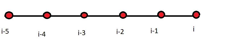 Let dx be the discretization size,we can second order approximation for fourth ORDER
`(del^(2)f)/(delx^(2))=``n.f(i-5)+p.f(i-4)+q.f(i-3)+r.f(i-2)+s.f(i-1)+t.f(i)`
| f(i) | f'(i) | f''(i) | `f^(3)(i)` | `f^(4)(i)` | `f^(5)(i)` | `f^(6)(i)` | |
| n.f(i-5) | n | -5n | 25n/2 | -125n/6 | 625n/24 | -3125n/120 | 15625n/720 |
| p.f(i-4) | p | -4p | 8p | -64p/6 | 256p/24 | -1024p/120 | 4096p/720 |
| q.f(i-3) | q | -3q | 9q/2 | -27q/6 | 81q/24 | -243q/120 | 729q/720 |
| r.f(i-2) | r | -2r | 2r | -8r/6 | 16r/24 | -32r/120 | 64r/720 |
| s.f(i-1) | s | -s | s/2 | -s/6 | s/24 | -s/120 | s/720 |
| t.f(i) | t | 0 | 0 | 0 | 0 | 0 | 0 |
|
`(del^(2)f)/(delx^(2))` =sum of above terms |
0 | 0 | 1 | 0 | 0 | 0 | will detemine |
n+p+q+r+s+t=0
-5n-4p-3q-2r-s=0
25n/2+8p+9q/2+2r+s/2=1
-125n/6-64p/6-27q/6-8r/6-s/6=0
625n/24+256p/24+81q/24+16r/24+s/24=0
-3125n/120-1024p/120-243q/120-32r/120-s/120=0
same like previosly the above equations represented in matrix form AX=B
`+o(dx)^(4)`
`[[1,1,1,1,1,1],[-5,-4,-3,-2,-1,0],[25/2,8,9/2,2,1/2,0],[-125/6,-64/6,-27/6,-8/6,-1/6,0],[625/24,256/24,81/24,2/3,1/24,0],[-3125/120,-1024/120,-81/40,-4/15,-1/120,0]]]``((n),(p),(q),(r),(s),(t))``=((0),(0),(1),(0),(0),(0))`
solving the above matrix
we will get n= -0.8333,p=5.0833,q=-13,r=17.8333,s=-12.8333,t=3.75
Finally if you substituted in above equation (2) and divided by `(dx)^(2)` we wil get
`(del^(2)f)/(delx^(2))=[n.f(i-5)+p.f(i-4)+q.f(i-3)+r.f(i-2)+s.f(i-1)+t.f(i)]/(dx)^(2)``+o(dx)^(4)`
MATLAB MAIN PROGRAMME
clear all
close all
clc
x=pi/3;
dx=linspace(pi/4000,pi/40,20);
 for i=1:length(dx)


   central_error(i)=fourth_order_approximations_center(x,dx(i));
   right_error(i)=fourth_order_approximations_right(x,dx(i));
    left_error(i)=fourth_order_approximations_left(x,dx(i));
end

 figure(1)
 loglog(dx,central_error,'b')
 hold on
 loglog(dx,right_error,'r')
 loglog(dx,left_error,'g')
 legend('central_error','right_error','left_error')
 xlabel('dx')
 ylabel('error')
Function codes
function[central_error]=fourth_order_approximations_center(x,dx)

%Given function f(x)=exp(x)*cos(x)
%Analytical second order derivative f''(x)=-2*exp(x)*sin(x)
analytical=-2*exp(x)*sin(x);

%Fourth order approximations f''(x)=a*f(i-2)+b*f(i-1)+c*f(i)+d*f(i+1)+e*f(i+2)/(dx)^(2)
% a,b,c,d,and e are coefficients calculated by taylors method

% AX=B
A = [1 1 1 1 1;-2 -1 0 1 2;2 0.5 0 0.5 2;-8/6 -1/6 0 1/6 8/6;2/3 1/24 0 1/24 2/3];
B= [0;0;1;0;0];
X = inv(A)*B;
a = X(1);
b = X(2);
c= X(3);
d= X(4);
e= X(5);

% a=-0.083333333333;
% b=1.333333333333;
% c=-2.5;
% d=1.333333333333;
% e=-0.083333333333;
Fourth_approximations_cen=( (a*exp(x-2*dx)*cos(x-2*dx)) + (b*exp(x-dx)*cos(x-dx)) + (c*exp(x)*cos(x)) + (d*exp(x+dx)*cos(x+dx)) + (e*exp(x+2*dx)*cos(x+2*dx)) )/(dx^2);
%Error

central_error=abs(Fourth_approximations_cen-analytical);
end
function[right_error]=fourth_order_approximations_right(x,dx)

%Given function f(x)=exp(x)*cos(x)
%Analytical second order derivative f''(x)=-2*exp(x)*sin(x)
analytical=-2*exp(x)*sin(x);
%Fourth order approximations
%f''(x)=g*f(i)+h*f(i+1)+j*f(i+2)+k*f(i+3)+l.f(i+4)+m.f(i+5)/(dx)^(2)
%g,h,j,k,l and m are coefficients calculated by taylors method
%CY=D
C=[1 1 1 1 1 1;0 1 2 3 4 5;0 0.5 2 4.5 8 12.5;0 1/6 8/6 27/6 64/6 125/6;0 1/24 2/3 81/24 256/24 625/24; 0 1/120 32/120 81/40 1024/120 3125/120];
D=[0;0;1;0;0;0];
Y=inv(C)*D;
g=Y(1);
h=Y(2);
j=Y(3);
k=Y(4);
l=Y(5);
m=Y(6);


% g=3.75;
% h=-12.833333333333;
% j=17.833333333333;
% k=-13;
% l=5.083333333333;
% m=-0.833333333333;
Fourth_approximations_right=( (g*exp(x)*cos(x)) + (h*exp(x+dx)*cos(x+dx)) + (j*exp(x+2*dx)*cos(x+2*dx)) + (k*exp(x+3*dx)*cos(x+3*dx)) + (l*exp(x+4*dx)*cos(x+4*dx)) + (m*exp(x+5*dx)*cos(x+5*dx)) )/(dx^2);
right_error=abs(Fourth_approximations_right-analytical);
end
function[left_error]=fourth_order_approximations_left(x,dx);
%Given function f(x)=exp(x)*cos(x)
%Analytical second order derivative f''(x)=-2*exp(x)*sin(x)
analytical=-2*exp(x)*sin(x);
%Fourth order approximations
%f''(x)=n*f(i-5)+p*f(i-4)+q*f(i-3)+r*f(i-2)+s.f(i-1)+t.f(i)/(dx)^(2)
%n,p,q,r,s and t are coefficients calculated by taylors method
%CY=D
E=[1 1 1 1 1 1;-5 -4 -3 -2 -1 0;25/2 8 9/2 2 1/2 0;-125/6 -64/6 -27/6 -8/6 -1/6 0;625/24 256/24 81/24 2/3 1/24 0;-3125/120 -1024/120 -81/40 -4/15 -1/120 0];
F=[0;0;1;0;0;0];
Z=inv(E)*F;
n=Z(1);
p=Z(2);
q=Z(3);
r=Z(4);
s=Z(5);
t=Z(6);
Fourth_approximations_left=( (n*exp(x-5*dx)*cos(x-5*dx)) + (p*exp(x-4*dx)*cos(x-4*dx)) + (q*exp(x-3*dx)*cos(x-3*dx)) + (r*exp(x-2*dx)*cos(x-2*dx)) + (s*exp(x-dx)*cos(x-dx)) + (t*exp(x)*cos(x)) )/(dx^2);
left_error=abs(Fourth_approximations_left-analytical);
end