Week 12 - Validation studies of Symmetry BC vs Wedge BC in OpenFOAM vs Analytical H.P equation
Objective:
- To simulate an axis-symmetric laminar flow through the constant cross-sectional of the pipe by applying the symmetry boundary condition.
- To simulating for the mentioned angles i.e for 10, 25, 45 degrees using both symmetry and wedge boundary conditions and validate them with HP equations.
Entrance length and Haigen-poiseuille equation
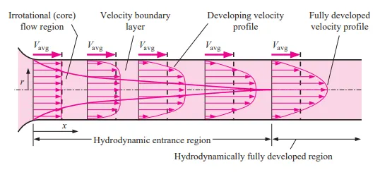
Consider a fluid entering a circular pipe at a uniform velocity. Because of the no-slip condition, the fluid particles in the layer in contact with the surface of the pipe come to a complete stop. This layer also causes the fluid particles in the adjacent layers to slow down gradually as a result of friction.To make up for this velocity reduction, the velocity of the fluid at the midsection of the pipe has to increase to keep the mass flow rate through the pipe constant. As a result, a velocity gradient develops along the pipe.
The region of the flow in which the effects of the viscous shearing forces caused by fluid viscosity are felt is called the velocity boundary layer or just the boundary layer. The hypothetical boundary surface divides the flow in a pipe into two regions: the boundary layer region, in which the viscous effects and the velocity changes are significant, and the irrotational (core) flow region, in which the frictional effects are negligible and thevelocity remains essentially constant in the radial direction.
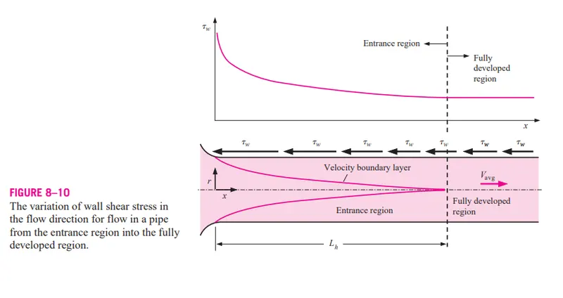
The thickness of this boundary layer increases in the flow direction until the boundary layer reaches the pipe center and thus fills the entire pipe, as shown in Fig. The region from the pipe inlet to the point at which the boundary layer merges at the centerline is called the hydrodynamic
entrance region, and the length of this region is called the hydrodynamic entry length Lh. Flow in the entrance region is called hydrodynamically developing flow since this is the region where the velocity profile develops.The region beyond the entrance region in which the velocity profile is fully developed and remains unchanged is called the hydrodynamically fullydeveloped region. The flow is said to be fully developed when the normalized temperature profile remains unchanged as well. Hydrodynamically developed flow is equivalent to fully developed flow when the fluid in the
pipe is not heated or cooled since the fluid temperature in this case remains essentially constant throughout. The velocity profile in the fully developed region is parabolic in laminar flow and somewhat flatter (or fuller) in turbulent flow due to eddy motion and more vigorous mixing in the radial direction.
The hydrodynamic entry length is usually taken to be the distance from the pipe entrance to where the wall shear stress (and thus the friction factor) reaches within about 2 percent of the fully developed value. In laminar flow,the hydrodynamic entry length is given approximately as `L_h=0.06ReD`
For a fully developed laminar flow the the pressur drop given by haigen-poiseuille equation is
`trianglep=(32muV_(avg)L)/D^(2)`
Similarly velocity profile in terms of average velocity `u(r)=2V_(avg)(1-r^(2)/R^(2))`
The average velocity in terms of pressure gradient given by `V_(avg)=-R^(2)/(8mu)(dp)/(dx)`
Also shear stress is given by`tau=mu(du)/(dy)`
where `mu`=Viscosity in N-s/m2
`V_(avg)`=Average velocity in m/s
L= Length of pipe in meters
D=Diameter of pipe in meters
R=Radius of pipe in meters
dp/dx=Pressure gradient
`L_h` = Hydrodynamic entrance length in meters
Re= Reynold number=2100
`tau`=Shear stress in N/m2
Procedure
1. The procedure for this challenge involves editing the previously made MATLAB code and changing the input and the Boundary Conditions in OpenFoam.
2. In the Automated BlockMeshDict file, we need to edit the wedge angle for one particular boundary condition. The angles at which we are performing the simulation are 10,25 and 45 degree.
MATLAB CODE
The code for symmetry boundary condition at angle of 25degrees is as follows(For wege condition we are replacing front and back type as wedge)
clear all
close all
clc

% User inputs
Re = 2100;

D = 0.02;
R=0.01;
rho = 1000;
mu = 0.89e-3;
theta = 25;
theta = theta/2;
fnb = 'symmetry';
z=0.3;

% Derived variables
Le = 0.06*Re*D;
nu = mu/rho;
L_developed = 0.3;
Lt = Le + L_developed;

%pressure and  velocity
v_avg=Re*mu/(D*rho);
v_max=2*v_avg;
del_P =(32*mu*v_avg*L_developed)/(D^2);
kin_P=del_P/rho;
r=linspace(0,0.01,100);
for i=1:length(r)
    tau(i)=0.5*r(i)*kin_P;
    x(i)=1-(r(i)/R)^(2);
    del_P =(32*mu*v_avg*L_developed)/(D^2);
kin_P=del_P/rho;
   v(i)=R^(2)*del_P*x(i)/(4*mu*L_developed);
   tau(i) = 4*mu*v_avg*(r(i))/R^2;
end
 z=linspace(0,0.3,30)
for j=1:length(z)
 del_P(j) =(32*mu*v_avg*z(j))/(D^2);
 kin_P(j)=del_P(j)/rho;
end
 figure(1)
 plot(r,tau,'LineWidth',2)
 xlabel('Radius')
 ylabel('Shear stress')
 legend('Shear stress of profile')
 hold on
 figure(2)
 plot(r,v,'LineWidth',2)
 xlabel('Radius')
 ylabel('Velocity')
 legend('Velocity profile')
 hold on
 figure(3)
 plot(z,kin_P,'LineWidth',2)
 xlabel('z')
 ylabel('Pressure drop')
 legend('Pressure profile')


f1=fopen('blockMeshDict','w')


% | \\      /  F ield         | OpenFOAM: The Open Source CFD Toolbox           |
% |  \\    /   O peration     | Version:  v2012                                 |
% |   \\  /    A nd           | Website:  www.openfoam.com                      |
% |    \\/     M anipulation  |                                                 |
% \*---------------------------------------------------------------------------*/
fprintf(f1,'%s \n','/*--------------------------------*- C++ -*----------------------------------*\');
fprintf(f1,'%s \n','| =========                 |                                                 |');
fprintf(f1,'%s \n','| \\      /  F ield         | OpenFOAM: The Open Source CFD Toolbox           |');
fprintf(f1,'%s \n','|  \\    /   O peration     | Version:  v2012                                 |');
fprintf(f1,'%s \n','|   \\  /    A nd           | Website:  www.openfoam.com                      |');
fprintf(f1,'%s \n','|    \\/     M anipulation  |                                                 |');
fprintf(f1,'%s \n','\*---------------------------------------------------------------------------*/');
fprintf(f1,'%s \n','FoamFile');
fprintf(f1,'%s \n','{');
fprintf(f1,'%s \n','version     2.0;');
fprintf(f1,'%s \n','format      ascii;');
fprintf(f1,'%s \n','class       dictionary;');
fprintf(f1,'%s \n','object      blockMeshDict;');
fprintf(f1,'%s \n','}');
fprintf(f1,'%s \n','// * * * * * * * * * * * * * * * * * * * * * * * * * * * * * * * * * * * * * //');
fprintf(f1,'%s \n','');


fprintf(f1,'scale\t 1;');
%vertices
fprintf(f1,'\nvertices');
fprintf(f1,'\n(');
fprintf(f1,'\n\t(%f\t%f\t%f)', 0, 0, 0);
fprintf(f1,'\n\t(%f\t%f\t%f)', 0, (D*cosd(theta)/2), (D*sind(theta)/2));
fprintf(f1,'\n\t(%f\t%f\t%f)', 0, (D*cosd(theta)/2), (-D*sind(theta)/2));
fprintf(f1,'\n\t(%f\t%f\t%f)', Lt, 0, 0);
fprintf(f1,'\n\t(%f\t%f\t%f)', Lt, (D*cosd(theta)/2), (D*sind(theta)/2));
fprintf(f1,'\n\t(%f\t%f\t%f)', Lt, (D*cosd(theta)/2), (-D*sind(theta)/2));
fprintf(f1,' \n);');

%blocks

fprintf(f1,'\nblocks');
fprintf(f1,'\n(');
fprintf(f1,' \n \t hex (0 3 5 2 0 3 4 1) (500 70 1) simpleGrading (1 1 1) ');
fprintf(f1,' \n);');

%edges

fprintf(f1,' \nedges');
fprintf(f1,'\n(');
fprintf(f1,' \n\tarc 1 2 (0\t\t0.01\t0)');
fprintf(f1,'\n\tarc 4 5 (2.82\t0.01\t0)');
fprintf(f1,'\n);');

%boundary inlet
fprintf(f1, '\nboundary\n');
fprintf(f1, '(\n');
fprintf(f1, '\t inlet \n');
fprintf(f1, '\t {\n');
fprintf(f1, '\t\t type patch;\n');
fprintf(f1, '\t\t faces\n');
fprintf(f1, '\t\t (\n');
fprintf(f1, '\t\t\t (0 1 2 0)\n');
fprintf(f1, '\t\t );\n');
fprintf(f1, '\t }\n');


%boundary outlet

fprintf(f1, '\t outlet \n');
fprintf(f1, '\t {\n');
fprintf(f1, '\t\t type patch;\n');
fprintf(f1, '\t\t faces\n');
fprintf(f1, '\t\t (\n');
fprintf(f1, '\t\t\t (3 5 4 3)\n');
fprintf(f1, '\t\t );\n');
fprintf(f1, '\t }\n');


%fixed wall

fprintf(f1, '\t top \n');
fprintf(f1, '\t {\n');
fprintf(f1, '\t\t type wall;\n');
fprintf(f1, '\t\t faces\n');
fprintf(f1, '\t\t (\n');
fprintf(f1, '\t\t\t (1 4 5 2)\n');
fprintf(f1, '\t\t );\n');
fprintf(f1, '\t }\n');

%front

fprintf(f1, '\t front \n');
fprintf(f1, '\t {\n');
fprintf(f1, '\t\t type %s;\n',fnb);
fprintf(f1, '\t\t faces\n');
fprintf(f1, '\t\t (\n');
fprintf(f1, '\t\t\t (0 3 4 1)\n');
fprintf(f1, '\t\t );\n');
fprintf(f1, '\t }\n');

%back
fprintf(f1, '\t back \n');
fprintf(f1, '\t {\n');
fprintf(f1, '\t\t type %s;\n',fnb);
fprintf(f1, '\t\t faces\n');
fprintf(f1, '\t\t (\n');
fprintf(f1, '\t\t\t (0 2 5 3)\n');
fprintf(f1, '\t\t );\n');
fprintf(f1, '\t }\n');

%axis
fprintf(f1, '\t axis \n');
fprintf(f1, '\t {\n');
fprintf(f1, '\t\t type empty;\n');
fprintf(f1, '\t\t faces\n');
fprintf(f1, '\t\t (\n');
fprintf(f1, '\t\t\t (0 3 3 0)\n');
fprintf(f1, '\t\t );\n');
fprintf(f1, '\t }\n');
fprintf(f1, ');\n');
fprintf(f1, 'mergePatchPairs\n');
fprintf(f1, '(\n');
fprintf(f1, ');\n');
fprintf(f1, '// ************************************************************************* //');
Explanation
1. Assign the initial values of the Hagen-Pousville flow.
2. Calculating the properties like dynamic viscocity, average velocity, maximum velocity, entrance length,kinematic pressure,pressure drop.
3. Calculate the shear stress, velocity profile and kinematic pressure drop by using for loop.
4. Plotting the values to obtain analytical solution.
Create BlockMeshDict file by using write function:
1. Assign vertices at all points on the wedge.
2. Drafting the blockMeshDict file using write function in MATLAB.
3. Drafting should be made with similar pattern as per the blockMeshDict file used in openFoam.
4. Writing the vertices of the wedge.
5. Creating the hexagonal block with simple grading
6. Assigning edges, wall, boundary, inlet, outlet, front and back of blocks.
Procedure to simulate the flow
1. Open terminal command in ubuntu.
2. open tutorials, code: tut
3. And open incompressible folder and select icofoam, then cavity. (code: icoFoam)
4. Copy cavity folder to run folder. using code: 'cp -r cavity/$FOAM_RUN/cavity_kohli
5. Type run command to open run folder.
6. Open pipe cavity_kohli (Also copy and paste the blockMeshDict file created by MATLAB in system folder)
7. Open system file.
8. Run blockMeshDict code file (code: blockMesh).
BlockMeshDict file
The blockMeshDict file for 25 degree of wedge with symmetrical boundry condition is as follows
/*--------------------------------*- C++ -*----------------------------------*\
| =========                 |                                                 |
| \\      /  F ield         | OpenFOAM: The Open Source CFD Toolbox           |
|  \\    /   O peration     | Version:  v2012                                 |
|   \\  /    A nd           | Website:  www.openfoam.com                      |
|    \\/     M anipulation  |                                                 |
\*---------------------------------------------------------------------------*/
FoamFile
{
version     2.0;
format      ascii;
class       dictionary;
object      blockMeshDict;
}
// * * * * * * * * * * * * * * * * * * * * * * * * * * * * * * * * * * * * * //

scale	 1;
vertices
(
	(0.000000	0.000000	0.000000)
	(0.000000	0.009763	0.002164)
	(0.000000	0.009763	-0.002164)
	(2.820000	0.000000	0.000000)
	(2.820000	0.009763	0.002164)
	(2.820000	0.009763	-0.002164)
);
blocks
(
 	 hex (0 3 5 2 0 3 4 1) (500 70 1) simpleGrading (1 1 1)
);
edges
(
	arc 1 2 (0		0.01	0)
	arc 4 5 (2.82	0.01	0)
);
boundary
(
	 inlet
	 {
		 type patch;
		 faces
		 (
			 (0 1 2 0)
		 );
	 }
	 outlet
	 {
		 type patch;
		 faces
		 (
			 (3 5 4 3)
		 );
	 }
	 top
	 {
		 type wall;
		 faces
		 (
			 (1 4 5 2)
		 );
	 }
	 front
	 {
		 type symmetry;
		 faces
		 (
			 (0 3 4 1)
		 );
	 }
	 back
	 {
		 type symmetry;
		 faces
		 (
			 (0 2 5 3)
		 );
	 }
	 axis
	 {
		 type empty;
		 faces
		 (
			 (0 3 3 0)
		 );
	 }
);
mergePatchPairs
(
);
// ************************************************************************* //
ControlDict file
/*--------------------------------*- C++ -*----------------------------------*\
| =========                 |                                                 |
| \\      /  F ield         | OpenFOAM: The Open Source CFD Toolbox           |
|  \\    /   O peration     | Version:  v2012                                 |
|   \\  /    A nd           | Website:  www.openfoam.com                      |
|    \\/     M anipulation  |                                                 |
\*---------------------------------------------------------------------------*/
FoamFile
{
    version     2.0;
    format      ascii;
    class       dictionary;
    location    "system";
    object      controlDict;
}
// * * * * * * * * * * * * * * * * * * * * * * * * * * * * * * * * * * * * * //

application     icoFoam;

startFrom       startTime;

startTime       0;

stopAt          endTime;

endTime         20;

deltaT          0.005;

writeControl    runTime;

writeInterval   0.1;

purgeWrite      0;

writeFormat     ascii;

writePrecision  6;

writeCompression off;

timeFormat      general;

timePrecision   6;

runTimeModifiable true;


// ************************************************************************* //
The velocity boundary conditions
/*--------------------------------*- C++ -*----------------------------------*\
| =========                 |                                                 |
| \\      /  F ield         | OpenFOAM: The Open Source CFD Toolbox           |
|  \\    /   O peration     | Version:  v2012                                 |
|   \\  /    A nd           | Website:  www.openfoam.com                      |
|    \\/     M anipulation  |                                                 |
\*---------------------------------------------------------------------------*/
FoamFile
{
    version     2.0;
    format      ascii;
    class       volVectorField;
    object      U;
}
// * * * * * * * * * * * * * * * * * * * * * * * * * * * * * * * * * * * * * //

dimensions      [0 1 -1 0 0 0 0];

internalField   uniform (0 0 0);

boundaryField
{
    inlet
    {
        type            fixedValue;
        value           uniform (0.0935 0 0);
    }

    outlet
    {
        type            zeroGradient;
    }

    top
    {
        type            noSlip;
    }

    front
    {
        type            symmetry;
    }

    back
    {
        type            symmetry;
    }
    axis
    {
        type            empty;
    }
}

// ************************************************************************* //
The pressure boundary conditions
/*--------------------------------*- C++ -*----------------------------------*\
| =========                 |                                                 |
| \\      /  F ield         | OpenFOAM: The Open Source CFD Toolbox           |
|  \\    /   O peration     | Version:  v2012                                 |
|   \\  /    A nd           | Website:  www.openfoam.com                      |
|    \\/     M anipulation  |                                                 |
\*---------------------------------------------------------------------------*/
FoamFile
{
    version     2.0;
    format      ascii;
    class       volScalarField;
    object      p;
}
// * * * * * * * * * * * * * * * * * * * * * * * * * * * * * * * * * * * * * //

dimensions      [0 2 -2 0 0 0 0];

internalField   uniform 0;

boundaryField
{
    inlet
    {
         type            zeroGradient;
    }

    outlet
    {

        type            fixedValue;
        value           uniform  1;
    }

    top
    {
        type            zeroGradient;
    }

    front
    {
        type            symmetry;
    }

    back
    {
        type            symmetry;
    }

    axis
    {
        type            empty;
    }
}


// ************************************************************************* //
Transport properties
/*--------------------------------*- C++ -*----------------------------------*\
| =========                 |                                                 |
| \\      /  F ield         | OpenFOAM: The Open Source CFD Toolbox           |
|  \\    /   O peration     | Version:  v2012                                 |
|   \\  /    A nd           | Website:  www.openfoam.com                      |
|    \\/     M anipulation  |                                                 |
\*---------------------------------------------------------------------------*/
FoamFile
{
    version     2.0;
    format      ascii;
    class       dictionary;
    location    "constant";
    object      transportProperties;
}
// * * * * * * * * * * * * * * * * * * * * * * * * * * * * * * * * * * * * * //

nu              8.9e-7;


// ************************************************************************* //
The Results of simulation
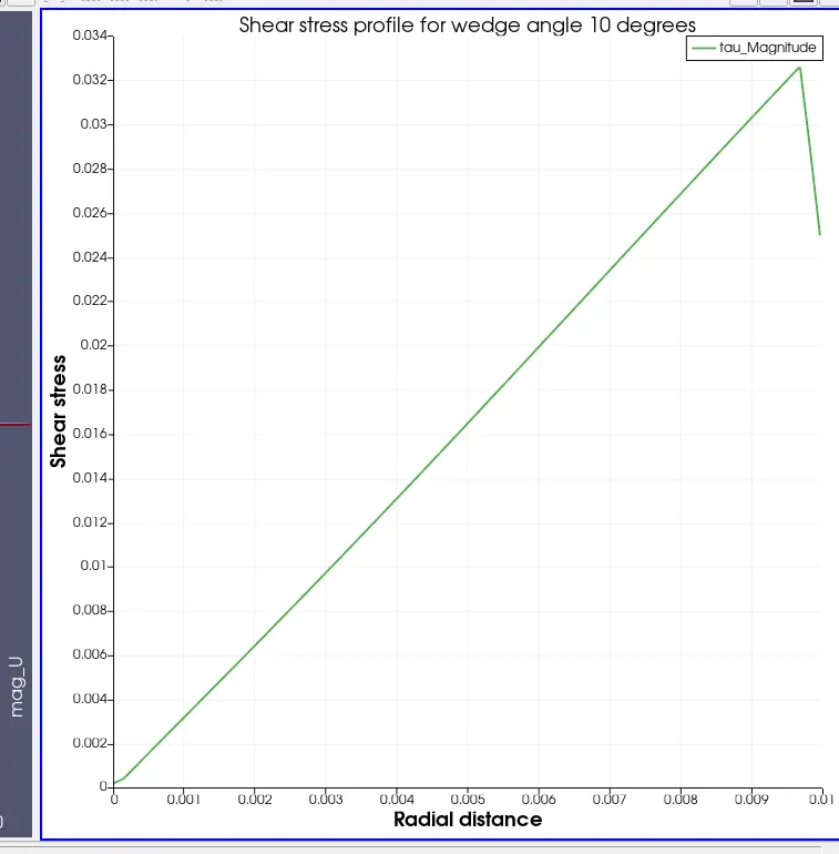
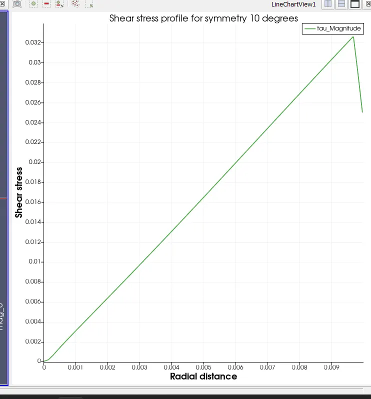
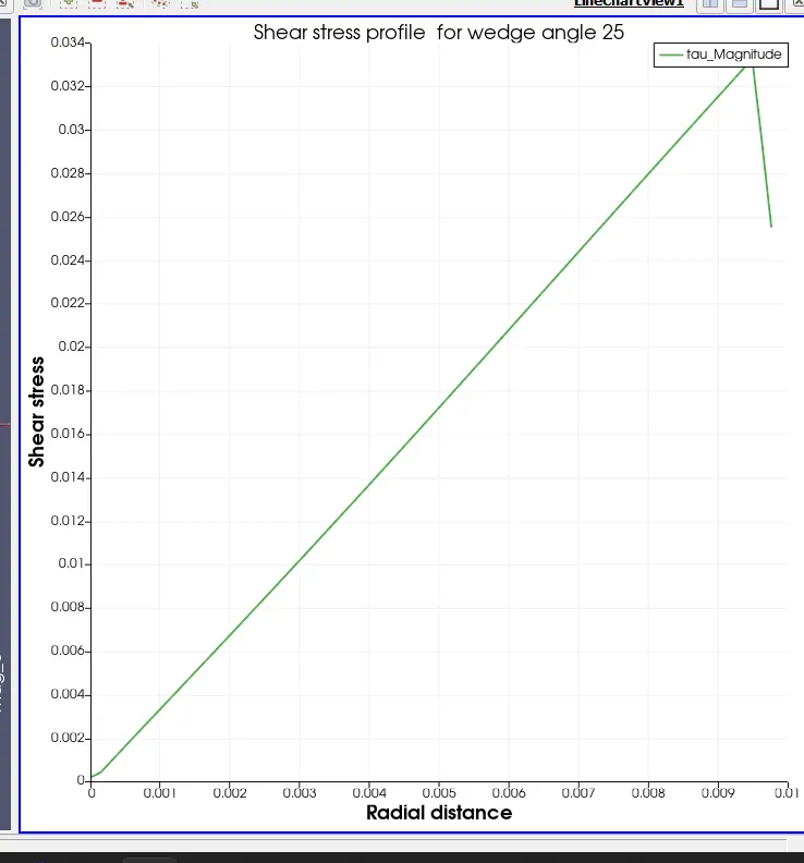
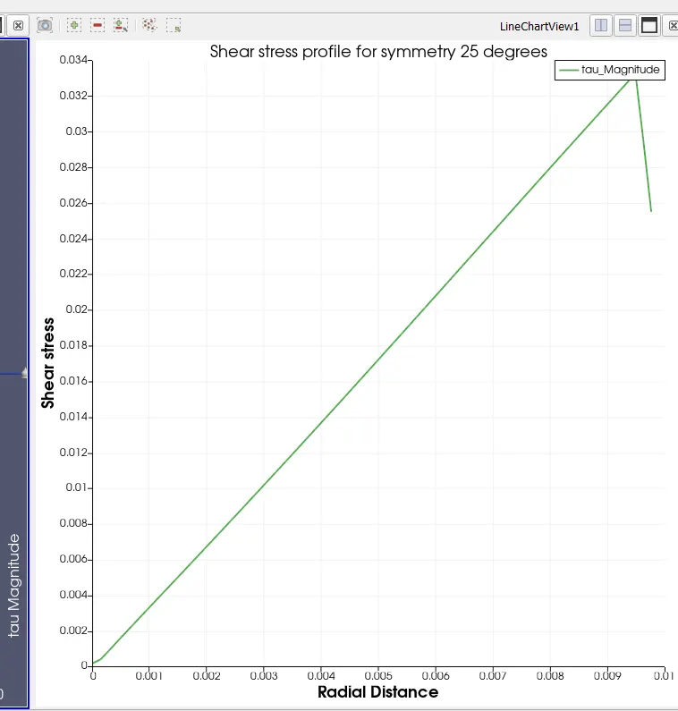
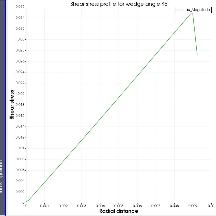
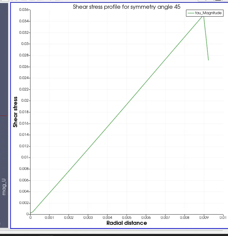
Shear stress developed for all angles(10,25 and 45) at both wedge and symmetry conditions
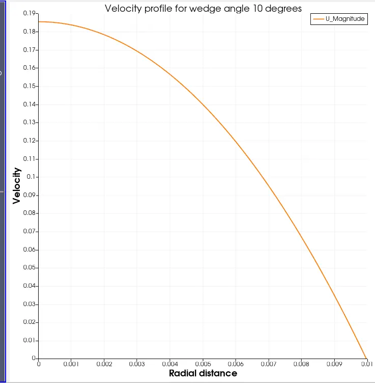
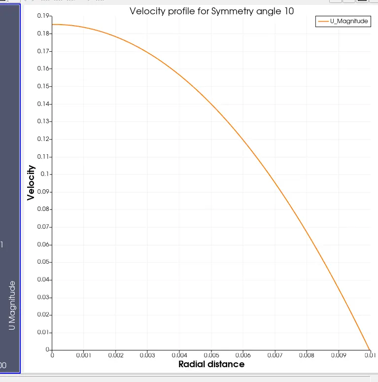
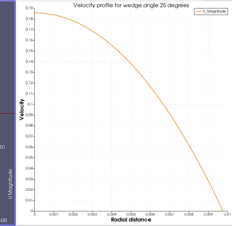
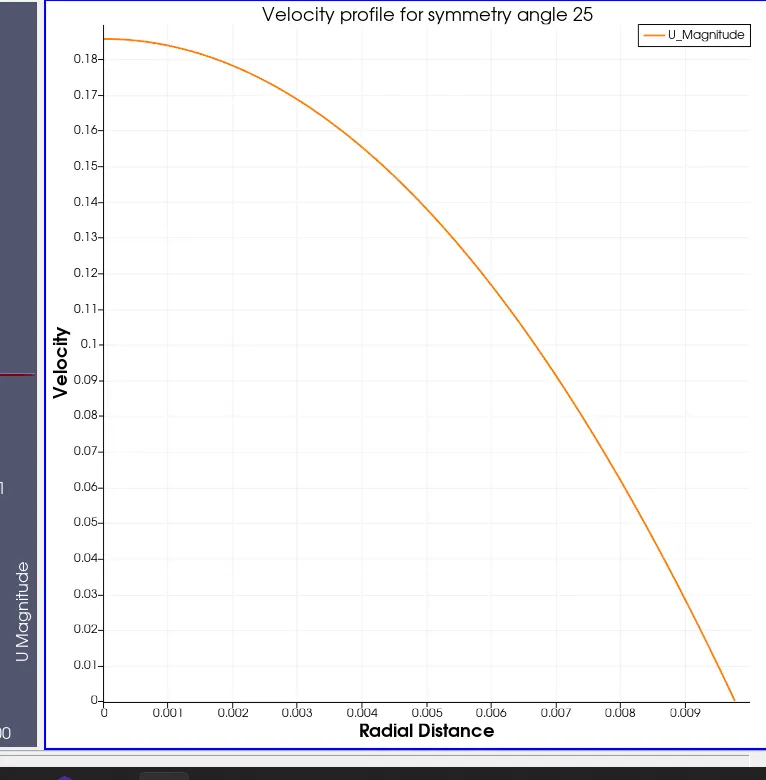
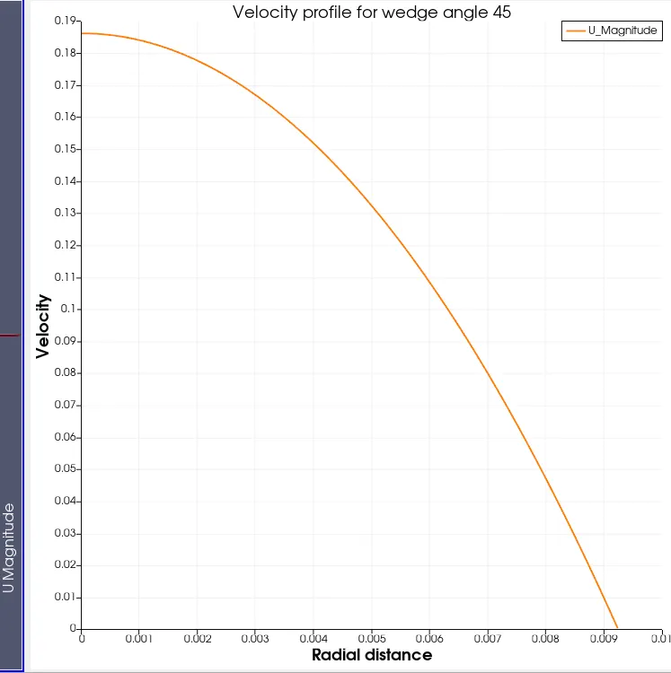
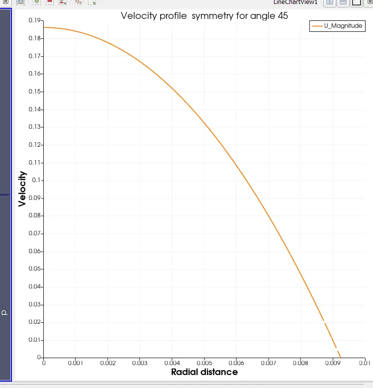
Velocity profile developed for all angles(10,25 and 45) at both wedge and symmetry conditions
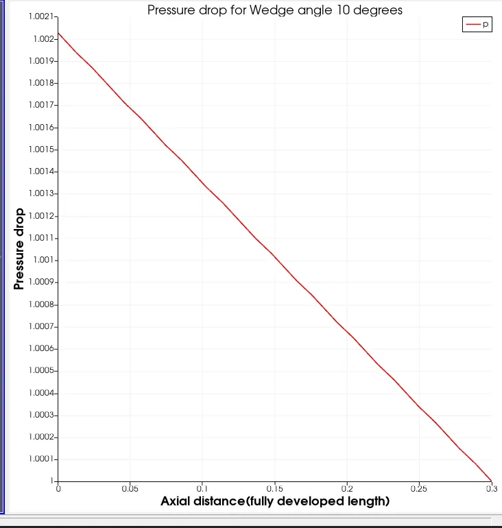
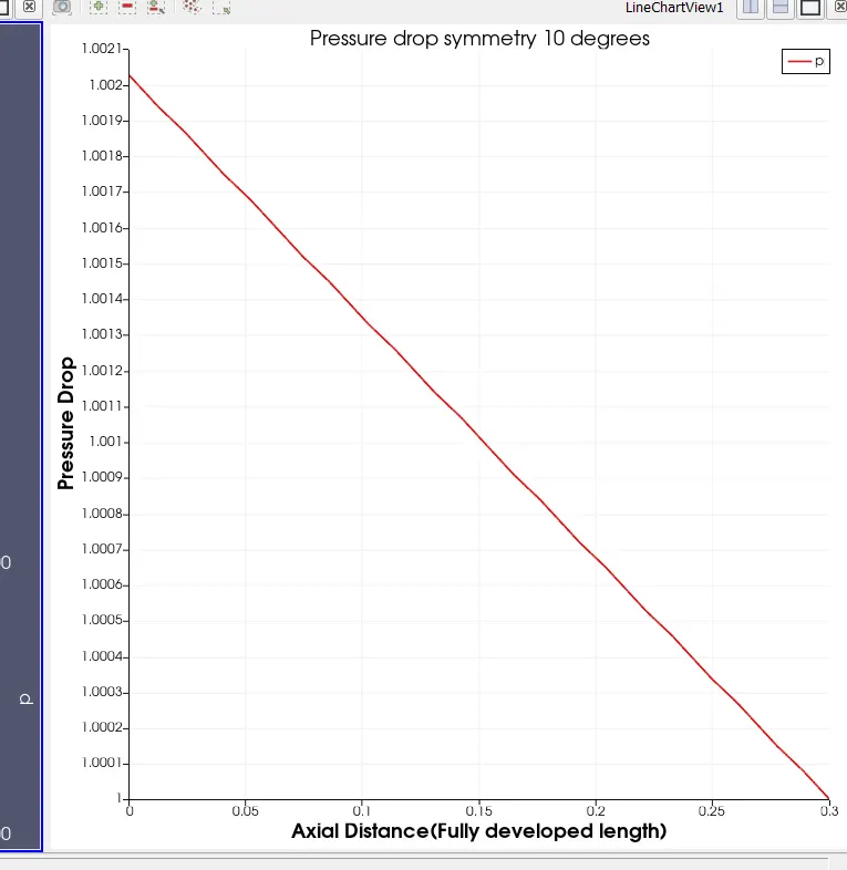
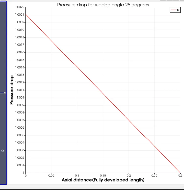
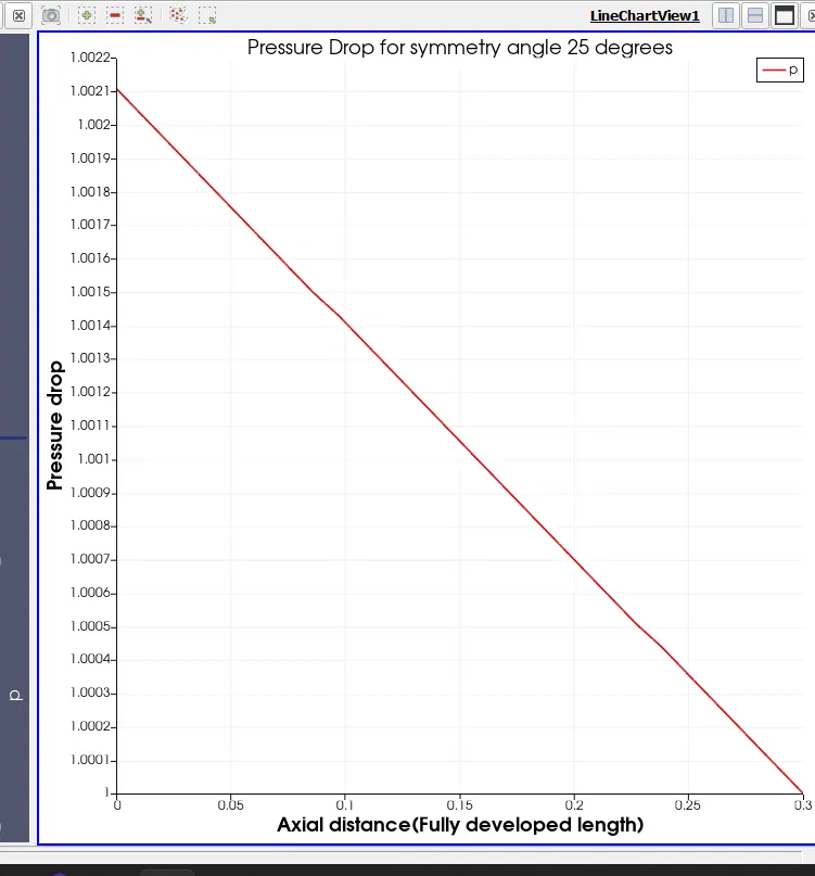
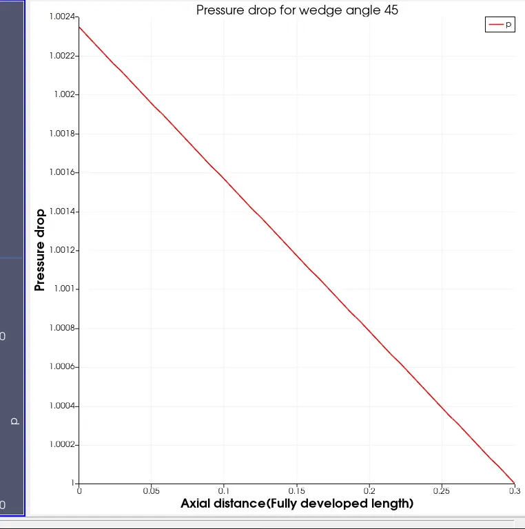
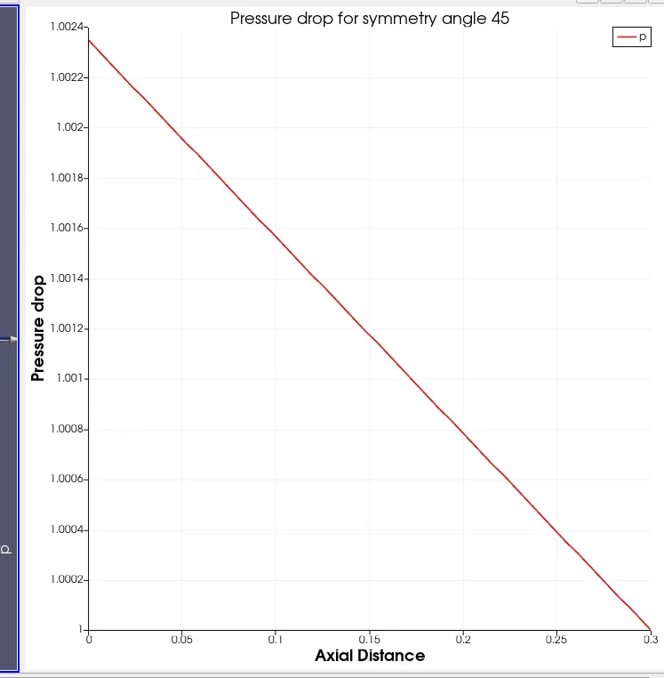
Pressure drop for all angles(10,25 and 45) at both wedge and symmetry conditions
Conclusions
1) Shear Stress is the maximum near the wall because of the friction that the wall has. But, as we move away from the wall, the Shear Force decreases, and it can be confirmed with the graph above. According to the Analytically calculated profile, the graph is`u(r)=2V_(avg)(1-r^(2)/(R^(2)))`And we know that this profile also gives out a Parabolic curve similar to the one we have gotten in the graph. For all angles both symmetry and wedge conditions we are getting almost similar results.
2) Now, If we wish to calculate the Hydrodynamic length analytically, the formula,`L_H=0.06ReD`
Re = Reynolds number.
D = Diameter.
In our case, Re = 2100 and the Diameter = 0.02m, so the Hydrodynamic Length is:
Lh = 0.06*2100*0.02 = 2.52m.
In all graphs, we can confirm that only after the Hydrodynamic length of approximately2.52m, the velocity profile is changing into a fully parabolic shape.
3) Pressure drop graphs are also same in both wedge and symmetry conditions for all angles.