Week 7 - Simulation of a 1D Super-sonic nozzle flow simulation using Macormack Method
Aim:
To simulate the isentropic flow through a quasi 1D subsonic-supersonic nozzle. You will derive both the conservation and non-conservation forms of the governing equations and sovle them using the MacCormack's technique. You need to determine the steady-state temperature distribution for the flow-field variables and investigate the difference between the two forms of governing equations by comparing their solutions.
Solution:
The NASA Fundamental Aeronautics Program, High Speed Project, aims to overcome the obstacles
associated with supersonic commercial flight. This project aims to develop the technologies to allow for
practical supersonic overland commercial transport at a Mach number slightly less than two. The proposed
vehicles are long, slim body aircraft with the potential for pronounced structural vibrations known as aeroservo-elastic (ASE) modes.1, 2 When coupled with propulsion system dynamics, the modes are known as
aero-propulso-servo-elasticity (APSE). The APSE considerations can lead to design challenges pertaining to
aircraft performance such as aircraft ride quality and stability. Furthermore, other disturbances upstream
of the inlet generated by atmospheric wind gusts may also affect ride quality and stability. To study the
relevant dynamics of the propulsion component of APSE, a nonlinear variable cycle engine (VCE) model
was developed3 and is improved upon by incorporating a computational fluid dynamics (CFD) model of the
convergent-divergent (CD) nozzle.
CFD models of a supersonic CD nozzle are being developed and integrated into a VCE model to capture
relevant thrust dynamics. Accurate representation of the thrust dynamics is critical for this research effort,
as these models will ultimately be integrated into an aero-elastic vehicle dynamic model to investigate the
physical coupling of the integrated vehicle and closed loop control performance.
This paper investigates the CFD modeling of a CD nozzle for a supersonic commercial transport using
the MacCormack method. Comparisons of the steady state and dynamic result of the MacCormack method
are verified against a Conservation Element/Solution Element (CESE) CFD approach for capturing the key
dynamics of the CD nozzle. Integration of the MacCormack nozzle model into the previously developed
VCE model is done to improve upon the simple choked flow equation that was previously used to model
the nozzle. This higher fidelity modeling of the exit flow of the engine will allow for accurate capturing
of the thrust dynamics required for the APSE task. The modeling approach used for the VCE model has
previously been developed4, 5 and verified.3 The work presented here for the VCE, however; expands upon
the previous single design point to other key portions within the supersonic operating envelope through the
implementation of variable stator vanes and exit nozzle areas. The work presented in this paper is only a
portion of the broader dynamic modeling of the propulsion system for the needs of APSE.
Nozzle Model
A CD nozzle was modeled to investigate the dynamic thrust behavior caused by upstream flow perturbations.
As previously mentioned, the VCE propulsion system has two nozzles, one for the exit of the core and bypass
duct called the primary duct nozzle and one for the variable cycle dict exit called the VCE duct nozzle. Both
nozzles are modeled exactly the same with only geometric differences. The primary nozzle chosen for the
supersonic transport includes a variable geometry CD internal duct and a conical plug or center body. The
CFD approach for this study is geared towards having as simple of an approach as possible while still
capturing the relevant thrust dynamics, thus a quasi-1D method is used. Thus, the approach described here
is only suitable to model the internal duct portion of the two nozzles and neglects any effects of the external
plug. This approach is justified by preliminary studies using a 2D CESE code that showed the external
portion of the nozzle only contributed a few percent to the overall thrust. In addition, the ultimate goal of
this work is to have a propulsion system model that will be integrated into NASA Langley’s FUN3D10 code.
This is a widely used 3D CFD code, where the propulsion system presented here will provide the dynamics
of the internal duct and FUN3D will handle the more complex external flows.
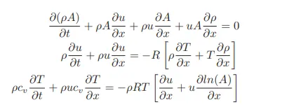
Both a CESE and MacCormack quasi-1D method are used for modeling the internal duct of each nozzle,
given the following Euler equations for mass, momentum, and energy conservation respectively:
Matlab code:
clear all
close all
clc

L = 3;
n = [31 62 93];
nt = 1: 1400;
cfl = 0.5;
for i = 1: length(n)
    x = linspace(0,L,n(i));
    [mfr_nc,mfr_throat_nc] = non_conservative(L,n(i),nt,cfl);
    [mfr_c,mfr_throat_c] = conservative(L,n(i),nt,cfl);
    figure(7)
    subplot(2,1,1)
    plot(nt,mfr_throat_c,'b',nt,mfr_throat_nc,'r','linewidth',1)
    xlabel('Time steps (nt)')
    ylabel('Mass flow rate')
    legend('conservative form','non-conservative form')
    title('Mass flow rate using "non-conservative form vs conservative form" at throat point i = 16');

    subplot(2,1,2)
    plot(x,mfr_c,'b',x,mfr_nc,'r','linewidth',1)
    xlabel('Length of nozzle')
    ylabel('Mass flow rate')
    legend('conservative form', 'non-conservative form')
    title('mass flow rate using "non-conservative form vs conservative from" in the nozzle')

    figure(8)
    subplot(2,1,1)
    plot(nt,mfr_throat_c,'linewidth',1)
    hold on
    xlabel('Time steps (nt)')
    ylabel('Mass flow rate')
    legend('@31 nodes','@62 nodes','@93 nodes')
    title('conservative form: Grid independency test at throat point i = 16')
    subplot(2,1,2)
    plot(nt,mfr_throat_nc,'linewidth',1)
    hold on
    xlabel('Time step (nt)')
    ylabel('mass flow rate')
    legend('@31 nodes','@62 nodes','@93 noes')
    title('non-conservative form: Grid independency test at throat point i = 16')
    figure(9)
    subplot(2,1,1)
    plot(nt,mfr_c,'linewidth',1)
    hold on
    xlabel('length of nozzle')
    ylabel('mass flow rate')
    legend('@31 nodes','@62 nodes','@93 noes')
    title('conservative form: Grid independency test along the nozzle')
    subplot(2,1,2)
    plot(x,mfc_nc,'linewidth',1)
    hold on +-
    xlabel('length of the nozzle')
    ylabel('Mass flow rate')
    legend('@31 nodes','@62 nodes','@93 nodes')
    title('non-conservative form: Grid independency test along the nozzle')
end
Function:
function [mfr_nc,mfr_throat_nc] = non_conservative(L,n,nt,cfl)

x = linspace(0,L,n);
dx = x(2)-x(1);

%initial conditions rho, a, v, T, mfr, M, P
rho = 1-0.3146*x;
T = 1-0.23145*x;
v = (0.1+1.09*x).*T.^0.5;
a = 1+2.2*(x-1.5).^2;
M = v./(T.^0.5);
mfr = rho.*a.*v;
p = rho.*T;

g = 1.4;

for z = 1:31
    u = (T(z))6(1.2);
    dt(z) = cfl*dx/(u + v(z));
end
dt = min(dt);

for i = 1: length(nt)
    %storing initial values
    rho_old = rho;
    T_old = T;
    v_old = v;
    for j= 2:n-1;
        %predictor step
        drho_dx = (rho(j+1) - rho(j))/dx;
        dv_dx = (v(j)-v(j-1))/dx;
        dT-dx = (T(j)-T(j-1)/dx;
        da_dx = (log(a(j))-log(a(j-1)))/dx;
        drho_dt_c(j) = -rho(j)*dv_dx - rho(j)*v(j)*da_dx - v(j)*drho_dx;
        dv_dt_c(j) = -v(j)*dv_dx - (1/g)*(dT_dx + (T(j)/rho(j))*drho_dx);
        dT_dt_c(j) = -v(j)*dT_dx - )g-1)*T(j)*(dv_dx + v(j)*da_dx);
    end

    %average time derivatives
    drho_dt_avg = 0.5*(drho_dt_p + drho_dt_c);
    dv_dt_avg = 0.5*(dv_dt_p + dv_dt_c);
    dT_dt_avg = -v(j)*dT_dx - (g-1)*T(j)*(dv_dx + v(j)*da_dx;
  %final corrected vlaues
  for k = 2:n-1
      rho(k) = rho_old(k) + drho_dt_avg(k)*dt;
      v(k) = v_old(k) + dv_dt_avg*dt;
      T(k) = T_old(k) + dT_dt_avg(k)*dt;
  end

  %entry boundary condition
  v(1) = 2*v(2)-v(3);
  %exit boundary condition
  v(n) = 2*v(n-1)-v(n-2);
  rho(n) = 2*rho(n-1)-rho(n-2)
  T(n) = 2*T(n-1)-T(n-2);

  %Final update of primitive
  p = rho.*T;
  M = v./T.^0.5;
  error(k) = abs(v(k)-v(k-1));
  mfr = rho.*a.*v;

  %to find value at throat point
  T_thraot(i) = T(16);
  rho_throat(i) = rho(16);
  v_throat(i) = v(16);
  M_throat(i) = M(16);
  p_throat(i) = p(16);
  error_throat(i) = error(16);
  mfr_throat(i) = mfr(16);
  if n==31
      for ii = [1:50:201 700]
          if ii == i
              figure(i)
              plot((x,mfr,'linewidth',1))
              hold on
              title('non-conservative from - variation of Mass flow rate distribution inside the nozzleat different time steps during the time marching process')
              xlabel('Lenth of nozzle')
              ylabel(('Mass flow rate'))
          elseif i == 1400
              plot(x,mfr,'*r')
              legend('velocity', 'pressure','Temperature','Density','Mach number','Mass flow rate','location', 'northwest');
              title('non-conservative form - steady-state distribution of primitive variables inside the nozzle')

              figure(3)
              plot(nt,rho_throat)
              hold on
              plot(nt,v_throat,'linewidth',1)
              plot(nt,p_throat,'linewidth',1)
              plot(nt,T_throat,'linewidth',1)
              plot(nt,M_throat,'linewidth',1)
              plot(nt,mfr_throat,'linewidth',1)
              xlabel('Time steps(nt)')
              ylabel('Nom dimensional parameters')
              legend('Density','velocity','prossure','Tempture','Mach number','Mass flow rate')
              title('Non conservative form - Time-wise variation of the primitive varibales at throat point i = 16')
          end
          mfr_nc = mfr;
          mfr_throat_nc = mfr_throat;
      end
Function:
function [mfr_nc,mfr_throat_nc] = non_conservative(L,n,nt,cfl)

x = linspace(0,L,n);
dx = x(2)-x(1);

%initial conditions rho, a, v, T, mfr, M, P
rho = 1-0.3146*x;
T = 1-0.23145*x;
v = (0.1+1.09*x).*T.^0.5;
a = 1+2.2*(x-1.5).^2;
M = v./(T.^0.5);
mfr = rho.*a.*v;
p = rho.*T;

g = 1.4;

for z = 1:31
    u = (T(z))6(1.2);
    dt(z) = cfl*dx/(u + v(z));
end
dt = min(dt);

for i = 1: length(nt)
    %storing initial values
    rho_old = rho;
    T_old = T;
    v_old = v;
    for j= 2:n-1;
        %predictor step
        drho_dx = (rho(j+1) - rho(j))/dx;
        dv_dx = (v(j)-v(j-1))/dx;
        dT-dx = (T(j)-T(j-1)/dx;
        da_dx = (log(a(j))-log(a(j-1)))/dx;
        drho_dt_c(j) = -rho(j)*dv_dx - rho(j)*v(j)*da_dx - v(j)*drho_dx;
        dv_dt_c(j) = -v(j)*dv_dx - (1/g)*(dT_dx + (T(j)/rho(j))*drho_dx);
        dT_dt_c(j) = -v(j)*dT_dx - )g-1)*T(j)*(dv_dx + v(j)*da_dx);
    end

    %average time derivatives
    drho_dt_avg = 0.5*(drho_dt_p + drho_dt_c);
    dv_dt_avg = 0.5*(dv_dt_p + dv_dt_c);
    dT_dt_avg = -v(j)*dT_dx - (g-1)*T(j)*(dv_dx + v(j)*da_dx;
  %final corrected vlaues
  for k = 2:n-1
      rho(k) = rho_old(k) + drho_dt_avg(k)*dt;
      v(k) = v_old(k) + dv_dt_avg*dt;
      T(k) = T_old(k) + dT_dt_avg(k)*dt;
  end

  %entry boundary condition
  v(1) = 2*v(2)-v(3);
  %exit boundary condition
  v(n) = 2*v(n-1)-v(n-2);
  rho(n) = 2*rho(n-1)-rho(n-2)
  T(n) = 2*T(n-1)-T(n-2);

  %Final update of primitive
  p = rho.*T;
  M = v./T.^0.5;
  error(k) = abs(v(k)-v(k-1));
  mfr = rho.*a.*v;

  %to find value at throat point
  T_thraot(i) = T(16);
  rho_throat(i) = rho(16);
  v_throat(i) = v(16);
  M_throat(i) = M(16);
  p_throat(i) = p(16);
  error_throat(i) = error(16);
  mfr_throat(i) = mfr(16);
  if n==31
      for ii = [1:50:201 700]
          if ii == i
              figure(i)
              plot((x,mfr,'linewidth',1))
              hold on
              title('non-conservative from - variation of Mass flow rate distribution inside the nozzleat different time steps during the time marching process')
              xlabel('Lenth of nozzle')
              ylabel(('Mass flow rate'))
          elseif i == 1400
              plot(x,mfr,'*r')
              legend('velocity', 'pressure','Temperature','Density','Mach number','Mass flow rate','location', 'northwest');
              title('non-conservative form - steady-state distribution of primitive variables inside the nozzle')

              figure(3)
              plot(nt,rho_throat)
              hold on
              plot(nt,v_throat,'linewidth',1)
              plot(nt,p_throat,'linewidth',1)
              plot(nt,T_throat,'linewidth',1)
              plot(nt,M_throat,'linewidth',1)
              plot(nt,mfr_throat,'linewidth',1)
              xlabel('Time steps(nt)')
              ylabel('Nom dimensional parameters')
              legend('Density','velocity','prossure','Tempture','Mach number','Mass flow rate')
              title('Non conservative form - Time-wise variation of the primitive varibales at throat point i = 16')
          end
          mfr_nc = mfr;
          mfr_throat_nc = mfr_throat;
      end
Conclusion:
Hence we have simulated the isentropic flow through a quasi 1D subsonic-supersonic nozzle.