Challenge

Project 2 - Rankine cycle Simulator

SSaquib Hazari19 Jan 2022

Aim:

To create a Rankin cycle stimulator using Matlab. To find the thermodynamic state points of each state.

Objective:

To Calculate the Rankin cycle State points at different stage.
To calculate the net work done by the system.
To find the Ratio of pump work.

Theory:

What is Rankin cycle:

The Rankine cycle is an idealized thermodynamic cycle describing the process by which certain heat engines, such as steam turbines or reciprocating steam engines, allow mechanical work to be extracted from a fluid as it moves between a heat source and heat sink

The Rankine cycle or Rankine Vapor Cycle is the process widely used by power plants such as coal plants or neuclear reactor. In this mechanism, a fuel is used to produce heat within a boiler, converting water into steam which then expands through a turbine producing useful work. This process was developed in 1859 by Scottish engineer William J.M. Rankine. This is a thermodynamic cycle which converts heat into mechanical energy—which usually gets transformed into electricity by electrical generation.

Pump:Compression of the fluid to high pressure using a pump (this takes work)
Boiler:The compressed fluid is heated to the final temperature (which is at boiling point), therefore, a phase change occurs—from liquid to vapor.
Turbine:Expansion of the vapor in the turbine.
Condenser:Condensation of the vapor in the condenser (where the waste heat goes to the final heat sink (the atmosphere or a large body of water (ex. lake or river).

The efficiency of the Rankine cycle is limited by the high heat of vaporization by the fluid. The fluid must be cycled through and reused constantly, therefore, is the water most practical fluid for this cycle. This is not why many power plants are located near a body of water that's for the waste heat.

As the water condenses in the condenser, is given off waste in the form of water vapour which can be seen billowing from a plant's cooling towers. This waste heat is necessary in any thermodynamic cycle. Due to this condensation step, the pressure at the turbine outlet is lowered. This means the pump requires less work to compress the water resulting in higher overall efficiencies.

Process:

Process 1-2: Isentropic expansion in the turbine.

Process 2-3: Isobaric cooling in the condenser.

Process 3-4: Isentropic compression in the pump.

Process 4-1: Isobaric heating in the boiler.

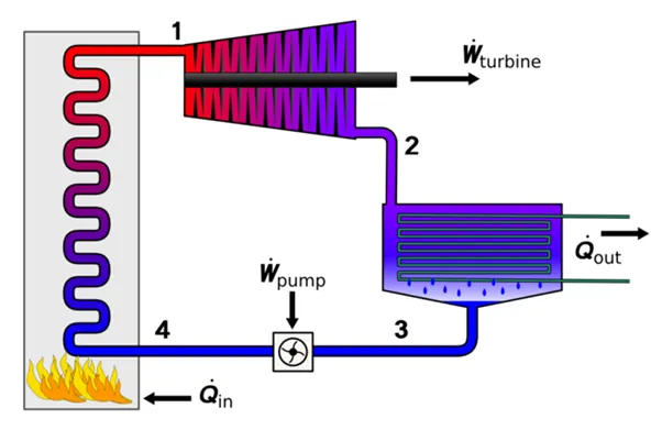
Equation applied is steady flow energy equation:

For boiler Q1 = h1 – hf4
For Turbine Wt = h1 – h2
For the Condenser Q2 = h2 – h3
For the feed pump Wp = hf4 – hf3
To calculate Efficiency => Eff = (Wt – Wp)/Q2
For the Net work done :
Wnet = Wp/Wt

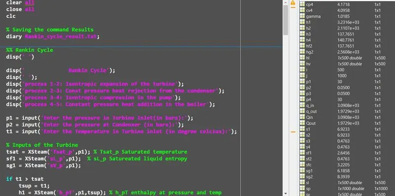
Main Code:

clear all

close all

clc

% Saving the command Results

diary Rankin_cycle_result.txt;

%% Rankin Cycle

disp(' ')

disp(' Rankin Cycle');

disp(' ');

disp('process 1-2: Isentropic expansion of the turbine');

disp('process 2-3: Const pressure heat rejection from the condenser');

disp('process 3-4: Isentropic compression in the pump');

disp('process 4-5: Constant pressure heat addition in the boiler');

p1 = input('Enter the pressure in Turbine Inlet(in bars):');

p2 = input('Enter the pressure at Condenser (in bars):');

t1 = input('Enter the Temperature in Turbine inlet (in degree celcius):');

% Inputs of the Turbine

tsat = XSteam('Tsat_p',p1); % Tsat_p Saturated temperature

sf1 = XSteam('sL_p',p1); % sL_p Satureated liquid entropy

sg1 = XSteam('sV_p',p1);

if t1 > tsat

tsup = t1;

h1 = XSteam('h_pT',p1,tsup); % h_pT enthalpy at pressure and temp

s1 = XSteam('s_pT',p1,tsup); % s_pT specific entropy at pressure and temp

elseif t1 == tsat

h1 = XSteam('hL_p',p1); % hL_p Saturated liquid enthalpy

s1 = XSteam('sL_p',p1); % sL_p Satureated liquid entropy

else

disp('Temperature must be greater than or equal to the saturation Temperature');

end

% Condenser Inlet

t2 = XSteam('Tsat_p', p2);

hf2 = XSteam('hL_p',p2);

hg2 = XSteam('hV_p',p2); % hV_p Saturated Volume enthalpy

s2 = s1;

sf2 = XSteam('sL_p',p2); % sL_p Satureated liquid entropy

sg2 = XSteam('sV_p',p2); % sV_p Saturated volume entopy

x2 = (s2 - sf2)/(sg2 - sf2);

h2 = hf2+(x2*(hg2 - hf2));

% Condenser exit

p3 = p2;

t3 = t2;

h3 = hf2;

s3 = sf2;

% Boiler Inlet

p4 = p1;

s4 = s3;

cp4 = XSteam('Cp_ps',p4,s4);

cv4 = XSteam('Cv_ps',p4,s4);

gamma = cp4/cv4;

t4 = t3*(p4/p3)^((gamma - 1)/gamma);

vf = XSteam('vL_p',p3); %vL_p Saturated liquid volume

wp = vf*(p1 - p2)*100;

h4 = wp + h3;

% Work done by turbine

wt = h1 - h2;

% Heat input

Qin = h1 - h4;

% Heat output;

Qout = h2 - h3;

% net work done

wnet = wt - wp;

% Thermal Efficiency

thermal_eff = (wnet/Qin)*100;

% Heat transfer to the boiler

q_in = h1 - h4;

% Heat rejected from the boiler

q_out = h2 - h3;

% Specific fuel consumption

sfc = 3600/wnet;

% Plotting T-S and H-S diagram;

% T-S diagram

figure(1)

hold on

% plotting of Saturation line

temp = linspace(1, 374, 500);

hl = zeros(1, 100);

hv = zeros(1, 100);

sl = zeros(1, 100);

sv = zeros(1, 100);

for i = 1 : length(temp)

hl(i) = XSteam('hL_T',temp(i));

hv(i) = XSteam('hV_T',temp(i));

sl(i) = XSteam('sL_T',temp(i));

sv(i) = XSteam('sV_T',temp(i));

end

plot(sl, temp, 'k', 'LineStyle','-','LineWidth', 1.5)

plot(sv, temp, 'k', 'LineStyle','-','LineWidth', 1.5)

xlabel('Specific Entropy (kJ/kgk)')

ylabel('Temperature (deg C)')

title('T-S diagram')

plot([s1 s2 s3 s4 sf1 sg2],[t1 t2 t3 t4 tsat tsat],"Color",'g','LineWidth',1.5);

text(s1,t1,'1');

text(s2,t2,'2');

text(s3,t3-10,'3')

text(s4,t4+10,'4')

t = linspace(tsat,tsup,1000);

for j = 1:length(t)

sp(j) = XSteam('s_pt',p1,t(j));

end

plot(sp,t,'Color','g','LineWidth',1.5);

% H-S diagram

figure(2)

hold on

plot(sl,hl,'r','LineStyle','-','LineWidth',1.5)

plot(sv,hv,'r','LineStyle','-','LineWidth',1.5)

plot([s1 s2 s3 s4 s1],[h1 h2 h3 h4 h1],'Color','black','LineWidth',1.5);

text(s1,h1,'1')

text(s2,h2,'2')

text(s3,h3-100,'3')

text(s4,h4+100,'4')

title('H-S diagram')

xlabel('Entropy (kJ/kgk)')

ylabel('Enthalpy (kJ/kg)')

%% Output

% at state 1

disp('Result');

disp('At state point 1')

fprintf('P1 is : %.2f Bar',p1);

fprintf('\n T1 is : %.2f Deg Celcius',t1);

fprintf('\n H1 is : %.2f (kJ/kg)',h1);

fprintf('\n S1 is : %.2f (kJ/kgK)\r\n',s1);

% at state 2

disp('Result');

disp('At state point 2')

fprintf('P2 is : %.2f Bar',p2);

fprintf('\n T2 is : %.2f Deg Celcius',t2);

fprintf('\n H2 is : %.2f (kJ/kg)',h2);

fprintf('\n S2 is : %.2f (kJ/kgK)\r\n',s2);

% at state 3

disp('Result');

disp('At state point 3')

fprintf('P3 is : %.2f Bar',p3);

fprintf('\n T3 is : %.2f Deg Celcius',t3);

fprintf('\n H3 is : %.2f (kJ/kg)',h3);

fprintf('\n S3 is : %.2f (kJ/kgK)\r\n',s3);

% at state 1

disp('Result');

disp('At state point 4')

fprintf('P4 is : %.2f Bar',p4);

fprintf('\n T4 is : %.2f Deg Celcius',t4);

fprintf('\n H4 is : %.2f (kJ/kg)',h4);

fprintf('\n S4 is : %.2f (kJ/kgK)\r\n',s4);

fprintf('Work output by turbine Wt is : %.2f kJ/kg',wt);

fprintf('\n Work input by the pump Wp is : %.2f kJ/kg',wp);

fprintf('\n Net work done Wnet is : %.2f kJ/kg',wnet);

fprintf('\n Thermodynamic eff is : %.2f percent',thermal_eff);

fprintf('\n Heat input by boiler : %.2f',q_in,' kJ/kg');

fprintf('\n Heat rejected by condenser : %.2f',q_out,' kJ/kg');

fprintf('\n Specific fuel consumption is : %.2f kg/Kwh',sfc);

Explanation:

Frist Displaying the Rankin cycle using disp command.
Using Disp command for displaying process takes place in Rankin cycle.
Now reading the Xsteam.m file provided carefully to obtain thermodynamic properties at different Stages.
When phase changes the temperature remains constant.
Calculating Net work, thermal efficiency, output and inputs all are displayed in the command prompt.
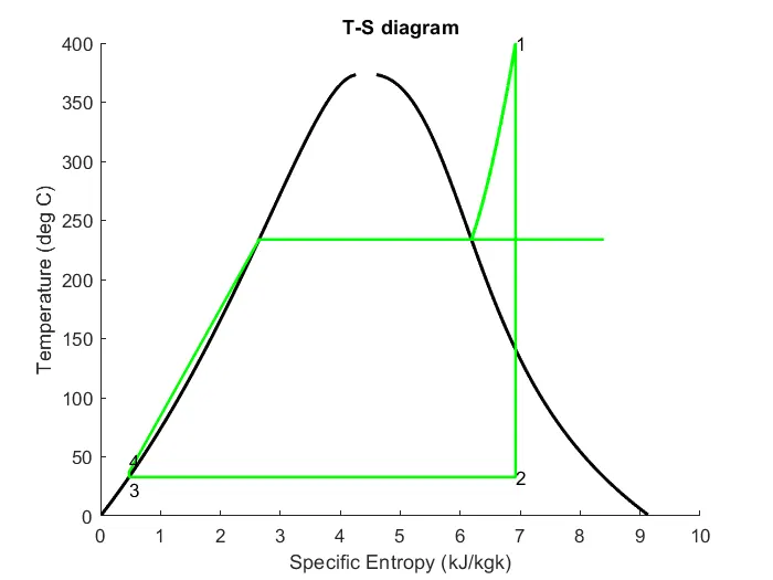
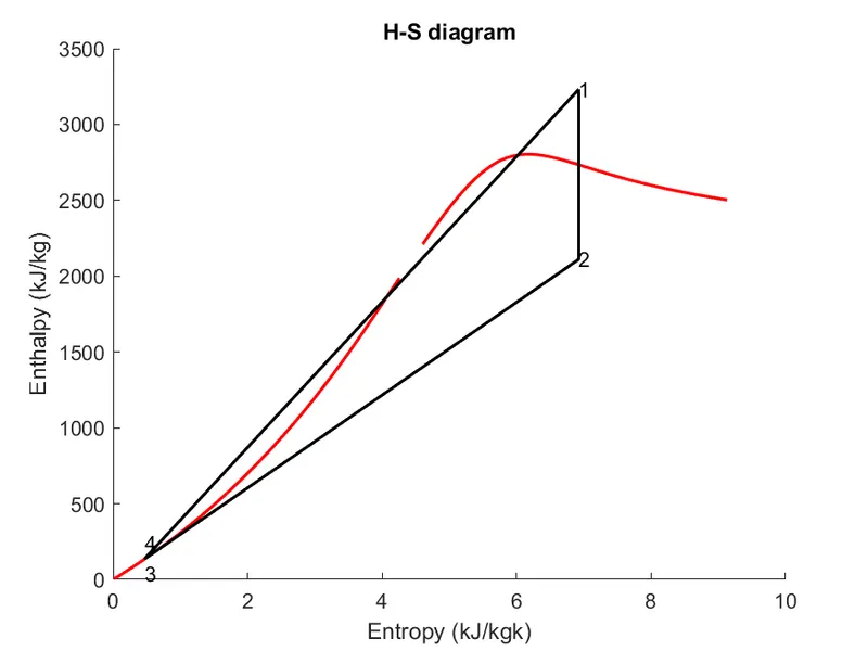
Now plotting the T-S and H-S diagram showing Entropy during the isobaric process.
Computing the variation of entropy during Isobaric process.
Displaying all the result at command window.
Generating .txt file by using Dairy command at the starting of the program.

Errors:

There were small syntax error which have been resolved immidiately.

Output:

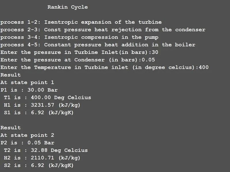
Rankin Cycle

process 1-2: Isentropic expansion of the turbine

process 2-3: Const pressure heat rejection from the condenser

process 3-4: Isentropic compression in the pump

process 4-5: Constant pressure heat addition in the boiler

Enter the pressure in Turbine Inlet(in bars):30

Enter the pressure at Condenser (in bars):0.05

Enter the Temperature in Turbine inlet (in degree celcius):400

Result

At state point 1

P1 is : 30.00 Bar

T1 is : 400.00 Deg Celcius

H1 is : 3231.57 (kJ/kg)

S1 is : 6.92 (kJ/kgK)

Result

At state point 2

P2 is : 0.05 Bar

T2 is : 32.88 Deg Celcius

H2 is : 2110.71 (kJ/kg)

S2 is : 6.92 (kJ/kgK)

Result

At state point 3

P3 is : 0.05 Bar

T3 is : 32.88 Deg Celcius

H3 is : 137.77 (kJ/kg)

S3 is : 0.48 (kJ/kgK)

Result

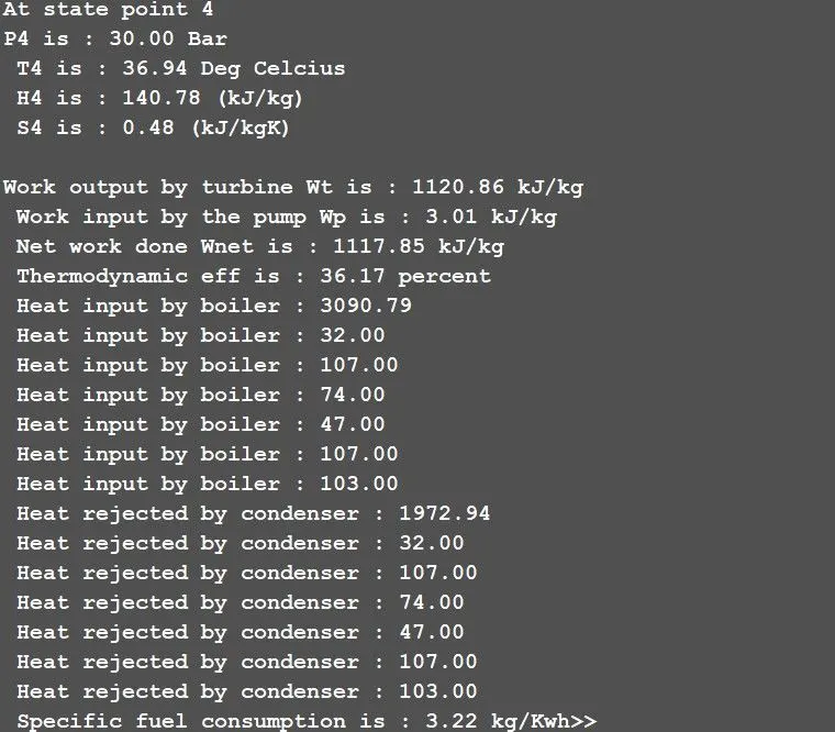
At state point 4

P4 is : 30.00 Bar

T4 is : 36.94 Deg Celcius

H4 is : 140.78 (kJ/kg)

S4 is : 0.48 (kJ/kgK)

Work output by turbine Wt is : 1120.86 kJ/kg

Work input by the pump Wp is : 3.01 kJ/kg

Net work done Wnet is : 1117.85 kJ/kg

Thermodynamic eff is : 36.17 percent

Heat input by boiler : 3090.79

Heat input by boiler : 32.00

Heat input by boiler : 107.00

Heat input by boiler : 74.00

Heat input by boiler : 47.00

Heat input by boiler : 107.00

Heat input by boiler : 103.00

Heat rejected by condenser : 1972.94

Heat rejected by condenser : 32.00

Heat rejected by condenser : 107.00

Heat rejected by condenser : 74.00

Heat rejected by condenser : 47.00

Heat rejected by condenser : 107.00

Heat rejected by condenser : 103.00

Specific fuel consumption is : 3.22 kg/Kwh

Plotting:

Reference:

https://en.wikipedia.org/wiki/Rankine_cycle

https://thereaderwiki.com/en/Rankine_cycle

https://energyeducation.ca/encyclopedia/Rankine_cycle

https://www.youtube.com/watch?v=Ec9kXfrZaR4

Project 2 - Rankine cycle Simulator

Ship work like this
in your own course.

Talk to a career counsellor

Ship work like thisin your own course.

Talk to a career counsellor

Ship work like this
in your own course.