Challenge

Week 4.1 - Genetic Algorithm

SSaquib Hazari9 Jan 2022

Aim: To optimise the stalagmite function and find the global maxima of the function.

Objective:

To explain the Genetic Algorithm with GA syntax.
To calculate the global maxima of stalagmite function.
To plot graph of various study cases.

Process:

Frist Creating Stalagmite function using the stalagmite governing equation.
Putting the stalagmite function in Ga syntax for optimise solution.
Plotting the graph and varying different study cases.

Theory:

Genetic Algorithm:

Nature has always been a great source of inspiration to all mankind. Genetic Algorithms (GAs) are search based algorithms based on the concepts of natural selection and genetics. GAs are a subset of a much larger branch of computation known as Evolutionary Computation.

GAs were developed by John Holland and his students and colleagues at the University of Michigan, most notably David E. Goldberg and has since been tried on various optimization problems with a high degree of success.

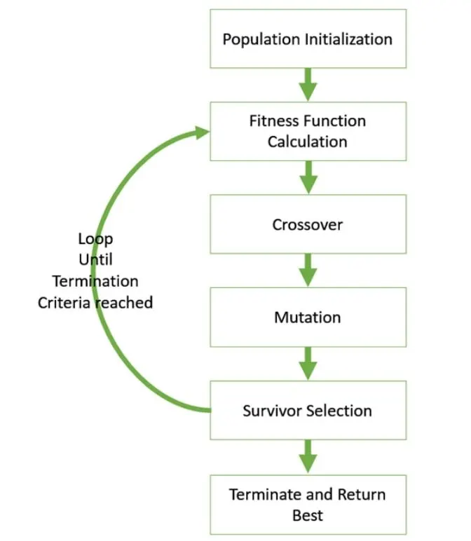
In GAs, we have a pool or a population of possible solutions to the given problem. These solutions then undergo recombination and mutation (like in natural genetics), producing new children, and the process is repeated over various generations. Each individual (or candidate solution) is assigned a fitness value (based on its objective function value) and the fitter individuals are given a higher chance to mate and yield more “fitter” individuals. This is in line with the Darwinian Theory of “Survival of the Fittest”.

In this way we keep “evolving” better individuals or solutions over generations, till we reach a stopping criterion.

Genetic Algorithms are sufficiently randomized in nature, but they perform much better than random local search (in which we just try various random solutions, keeping track of the best so far), as they exploit historical information as well.

GA:

The genetic algorithm is a method for solving both constrained and unconstrained optimization problems that is based on natural selection, the process that drives biological evolution. The genetic algorithm repeatedly modifies a population of individual solutions. At each step, the genetic algorithm selects individuals at random from the current population to be parents and uses them to produce the children for the next generation. Over successive generations, the population "evolves" toward an optimal solution. You can apply the genetic algorithm to solve a variety of optimization problems that are not well suited for standard optimization algorithms, including problems in which the objective function is discontinuous, nondifferentiable, stochastic, or highly nonlinear. The genetic algorithm can address problems of mixed integer programming, where some components are restricted to be integer-valued.

The genetic algorithm uses three main types of rules at each step to create the next generation from the current population:

Selection rules select the individuals, called parents, that contribute to the population at the next generation.
Crossover rules combine two parents to form children for the next generation.
Mutation rules apply random changes to individual parents to form children.

Advantages of GAs:

Does not require any derivative information (which may not be available for many real-world problems).
Is faster and more efficient as compared to the traditional methods.
Has very good parallel capabilities.
Optimizes both continuous and discrete functions and also multi-objective problems.
Provides a list of “good” solutions and not just a single solution.
Always gets an answer to the problem, which gets better over the time.
Useful when the search space is very large and there are a large number of parameters involved.

Limitations of GAs:

GAs are not suited for all problems, especially problems which are simple and for which derivative information is available.
Fitness value is calculated repeatedly which might be computationally expensive for some problems.
Being stochastic, there are no guarantees on the optimality or the quality of the solution.
If not implemented properly, the GA may not converge to the optimal solution.

Population:

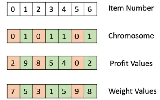
Population is a subset of solutions in the current generation. It can also be defined as a set of chromosomes. There are several things to be kept in mind when dealing with GA population −

The diversity of the population should be maintained otherwise it might lead to premature convergence.
The population size should not be kept very large as it can cause a GA to slow down, while a smaller population might not be enough for a good mating pool. Therefore, an optimal population size needs to be decided by trial and error.

The population is usually defined as a two dimensional array of – size population, size x, chromosome size.

Fitness function:

A fitness function simply defined is a function which takes the solution as input and produces the suitability of the solution as the output. In some cases, the fitness function and the objective function may be the same, while in others it might be different based on the problem.

Calculation of fitness value is done repeatedly in a GA and therefore it should be sufficiently fast. A slow computation of the fitness value can adversely affect a GA and make it exceptionally slow.

In most cases the fitness function and the objective function are the same as the objective is to either maximize or minimize the given objective function. However, for more complex problems with multiple objectives and constraints, an Algorithm Designer might choose to have a different fitness function.

Crossover:

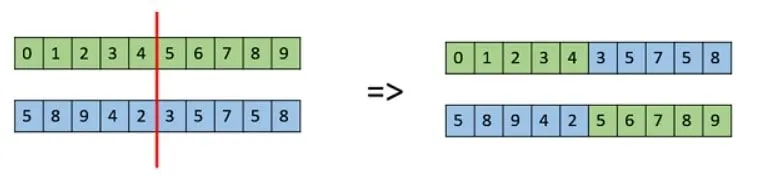
The crossover operator is analogous to reproduction and biological crossover. In this more than one parent is selected and one or more off-springs are produced using the genetic material of the parents. Crossover is usually applied in a GA with a high probability – p_c .

Single Point Crossover : A crossover point on the parent organism string is selected. All data beyond that point in the organism string is swapped between the two parent organisms. Strings are characterized by Positional Bias.

Two-Point Crossover : This is a specific case of a N-point Crossover technique. Two random points are chosen on the individual chromosomes (strings) and the genetic material is exchanged at these points.

Mutation:

In simple terms, mutation may be defined as a small random tweak in the chromosome, to get a new solution. It is used to maintain and introduce diversity in the genetic population and is usually applied with a low probability – p_m. If the probability is very high, the GA gets reduced to a random search.

Mutation is the part of the GA which is related to the “exploration” of the search space. It has been observed that mutation is essential to the convergence of the GA while crossover is not.

Termination:

The termination condition of a Genetic Algorithm is important in determining when a GA run will end. It has been observed that initially, the GA progresses very fast with better solutions coming in every few iterations, but this tends to saturate in the later stages where the improvements are very small. We usually want a termination condition such that our solution is close to the optimal, at the end of the run.

Stalagmite function:

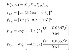
function [f] = stalagmite_func(input_vector)

 x = input_vector(1);
 y = input_vector(2);

 term1 = (sin(5.1*pi*x + 0.5))^6;

 term2 = (sin(5.1*pi*y + 0.5))^6;

 m1 = ((x - 0.0667)^2/(0.64));     % Solving the second part of eq
 m2 = ((y - 0.0667)^2/(0.64));      %Solving the second part of eq
 
 term3 = exp(-4*log(2)*m1);
 term4 = exp(-4*log(2)*m2);
 
 f = -1*(term1*term2*term3*term4);  % negative means it is inverted.
end

Explaining the GA syntax:

fun — Objective function:

Objective function, specified as a function handle or function name. Write the objective function to accept a row vector of length nvars and return a scalar value.

When the 'Use Vectorized' option is true, write fun to accept a pop-by-nvars matrix, where pop is the current population size. In this case, fun returns a vector the same length as pop containing the fitness function values. Ensure that fun does not assume any particular size for pop, since ga can pass a single member of a population even in a vectorized calculation.

nvars — Number of variables:

Number of variables, specified as a positive integer. The solver passes row vectors of length nvars to fun.

A — Linear inequality constraints:

Linear inequality constraints, specified as a real matrix. A is an M-by-nvars matrix, where M is the number of inequalities.

A encodes the M linear inequalities

A*x <= b,

b — Linear inequality constraints:

Linear inequality constraints, specified as a real vector. b is an M-element vector related to the a matrix. If you pass b as a row vector, solvers internally convert b to the column vector b(:).

b encodes the M linear inequalities

A*x <= b,

Aeq — Linear equality constraints:

Linear equality constraints, specified as a real matrix. Aeq is an Me-by nvars matrix, where Me is the number of equalities.

Aeq encodes the Me linear equalities

Aeq*x = beq,

beq — Linear equality constraints:

Linear equality constraints, specified as a real vector. beq is an Me-element vector related to the aeq matrix. If you pass beq as a row vector, solvers internally convert beq to the column vector beq(:).

beq encodes the Me linear equalities

Aeq*x = beq,

lb — Lower bounds:

Lower bounds, specified as a real vector or array of doubles. lb represents the lower bounds element-wise in lb ≤ x ≤ ub.

Internally, ga converts an array lb to the vector lb(:).

ub — Upper bounds:

Upper bounds, specified as a real vector or array of doubles. ub represents the upper bounds element-wise in lb ≤ x ≤ ub.

Internally, ga converts an array ub to the vector ub(:).

nonlcon — Nonlinear constraints

Nonlinear constraints, specified as a function handle or function name. nonlcon is a function that accepts a vector or array x and returns two arrays, c(x) and ceq(x).

c(x) is the array of nonlinear inequality constraints at x. ga attempts to satisfy

c(x) <= 0

for all entries of c.

ceq(x) is the array of nonlinear equality constraints at x. ga attempts to satisfy

ceq(x) = 0

for all entries of ceq.

options — Optimization options

Optimization options, specified as the output of optimoptions or a structure.

Code:

Case I:

clear all 
close all 
clc

%% Study:1 Static behaviour without bounds

% Inputs
x = linspace(0,0.6,150);
y = linspace(0,0.6,150);
num_cases = 100;          % Number of iteration

% 2d Mesh grid
[x,y] = meshgrid(x,y);

% Evaluating stalagmite value
for i = 1:length(x)
    for j = 1:length(y)
        input_vector(1) = x(i,j);                   %Creating Arrays
        input_vector(2) = y(i,j);
        f(i,j) = stalagmite_func(input_vector);     %using the stalagmite func that have been created
    end
end

tic
for i = 1:num_cases                                    % finding for each no of iteration
    [inputs, fopt(i)] = ga(@stalagmite_func,2);   % calling the stalagmite function
    xopt(i) = inputs(1);
    yopt(i) = inputs(2);
end
lap1_time = toc

% Plotting the function
subplot(2,1,1);           %subplot having two plot in same fig
hold on;
surfc(x,y,f);             %Inverting the stalagmite plot
shading interp;            %shading on to remove the mesh
plot3(xopt,yopt,fopt,'Marker','o','MarkerSize',5,'MarkerFaceColor','r');  %Maker creates circle at the pick of minima
xlabel('x-axis');
ylabel('y-axis');
title('unbound inputs');
subplot(2,1,2);
plot(fopt);
xlabel('Iteration');
ylabel('Function minimum');

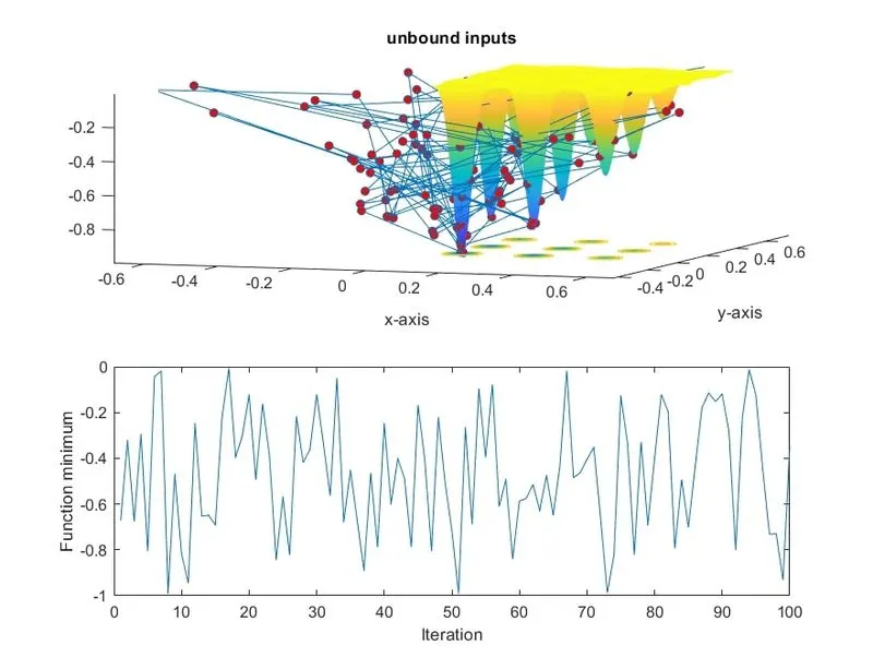
Result: In this case study without bounds there are various random values which indicates that our solution is wrong, and we have to modify the eq further.

Case II:

%% Study: 2  Static behaviour with bounds

% Inputs
x = linspace(0,0.6,150);
y = linspace(0,0.6,150);
num_cases = 100;          % Number of iteration

% 2d Mesh grid
[x,y] = meshgrid(x,y);

% Evaluating stalagmite value
for i = 1:length(x)
    for j = 1:length(y)
        input_vector(1) = x(i,j);
        input_vector(2) = y(i,j);
        f(i,j) = stalagmite_func(input_vector);
    end
end

tic

% Inputs functions
%fun = @stalagmit_fun
%navrs = 2
%A = []
%b = []
%Aeq = []
%beq = []
%lb = [0;0]
%ub = [0.1;0.1]
%nonlcon = []
%Intcon = []

for i = 1:num_cases                                    % finding for each no of iteration
    [inputs, fopt(i)] = ga(@stalagmite_func,2,[],[],[],[],[0;0],[0.6;0.6]);   % calling the stalagmite function
    xopt(i) = inputs(1);
    yopt(i) = inputs(2);
end
lap2_time = toc

% Plotting the function
subplot(2,1,1);           %subplot having two plot in same fig
hold on;
surfc(x,y,f);             %Inverting the stalagmite plot
shading interp;            %shading on to remove the mesh
plot3(xopt,yopt,fopt,'Marker','o','MarkerSize',5,'MarkerFaceColor','r');
xlabel('x-axis');
ylabel('y-axis');
title('bound inputs');
subplot(2,1,2);
plot(fopt);
xlabel('Iteration');
ylabel('Function minimum');

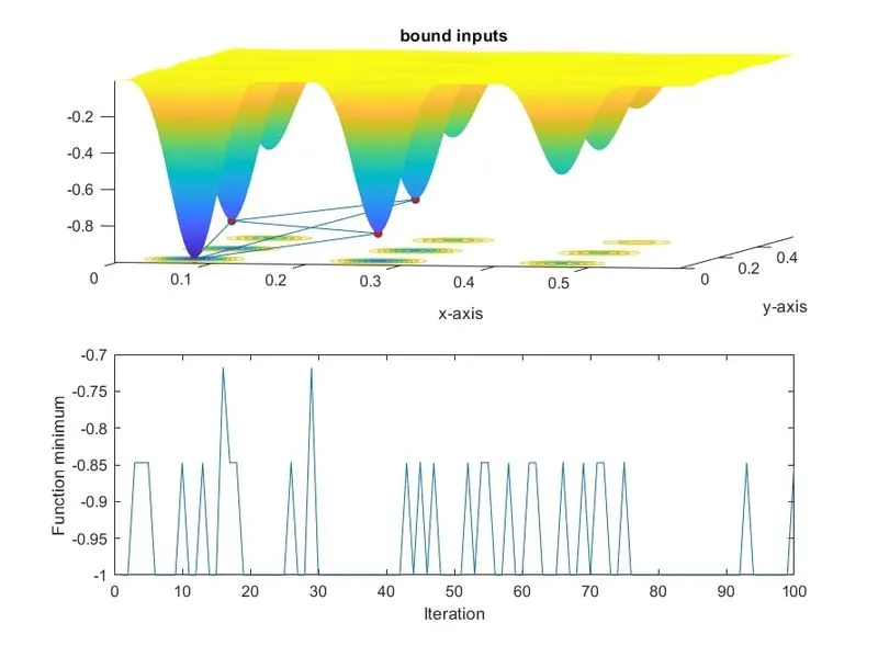
Result: In second case study we have achieve 4 Global minima points with bounds which indicates our solution is right by can be further modifies unless we get our solution.

Case III:

%% Stydy: 3 Static behaviour with bounds and larger population

% Inputs
x = linspace(0,0.6,150);
y = linspace(0,0.6,150);
num_cases = 100;          % Number of iteration

% 2d Mesh grid
[x,y] = meshgrid(x,y);

% Evaluating stalagmite value
for i = 1:length(x)
    for j = 1:length(y)
        input_vector(1) = x(i,j);
        input_vector(2) = y(i,j);
        f(i,j) = stalagmite_func(input_vector);
    end
end

% Now increasing the population

tic
options = optimoptions('ga');
options = optimoptions(options,'PopulationSize',170);  %increasing the size on the population

% Inputs functions
%fun = @stalagmit_fun
%navrs = 2
%A = []
%b = []
%Aeq = []
%beq = []
%lb = [0;0]
%ub = [0.1;0.1]
%nonlcon = []
%Intcon = []

for i = 1:num_cases                                    % finding for each no of iteration
    [inputs, fopt(i)] = ga(@stalagmite_func,2,[],[],[],[],[0;0],[0.1;0.1],[],[]);   % calling the stalagmite function
    xopt(i) = inputs(1);
    yopt(i) = inputs(2);
end
lap2_time = toc

% Plotting the function
subplot(2,1,1);           %subplot having two plot in same fig
hold on;
surfc(x,y,-f);             % Again Inverting the stalagmite plot
shading interp;            %shading on to remove the mesh
plot3(xopt,yopt,-fopt,'Marker','o','MarkerSize',5,'MarkerFaceColor','r');
xlabel('x-axis');
ylabel('y-axis');
title('bound inputs with larger population');
subplot(2,1,2);
plot(-fopt);
xlabel('Iteration');
ylabel('Function minimum');

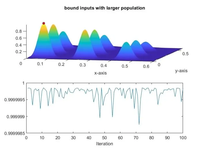
Result: our third case study with bounds and increase in population has given the exact value which we are looking for, the value of Global maxima is '1'.

Explaining the Code:

Defining the workspace and no of iteration.
Creation of 2D mesh gird.
Defining the no of cases.
Defining the stalagmite function inside the loop.
Creating the surf plot.
For each iteration generation the Ga solution.
Plotting the stalagmite function at maximum value.

Errors:

Minute syntactic errors which resolved immediately.

References:

Week 4.1 - Genetic Algorithm

nvars — Number of variables:

A — Linear inequality constraints:

b — Linear inequality constraints:

Aeq — Linear equality constraints:

beq — Linear equality constraints:

lb — Lower bounds:

ub — Upper bounds:

nonlcon — Nonlinear constraints

options — Optimization options

Ship work like this
in your own course.

Talk to a career counsellor

nvars — Number of variables:

A — Linear inequality constraints:

b — Linear inequality constraints:

Aeq — Linear equality constraints:

beq — Linear equality constraints:

lb — Lower bounds:

ub — Upper bounds:

nonlcon — Nonlinear constraints

options — Optimization options

Ship work like thisin your own course.

Talk to a career counsellor

Ship work like this
in your own course.