Week 11 - Simulation of Flow through a pipe in OpenFoam
Objectives:
- Calculation of Flow Variables
- Generation of blockMeshDict using the wedge boundary condition. Create the blockMeshDict file in MATLAB such that the mesh is
automatically created for any wedge angle. - Simulating the pipe flow in OpenFOAM using icoFoam solver.
- Post process the velocity profile and shear stress and compare the simulation results with analytical results obtained using the
Hagen-Poiseuille equation.
Entrance Length:
The length of the entrance is the distance that fluid travels after entering a pipe before the full development of the flow. Entrance
length refers to the length of the entry region, where effects from the pipe's interior wall spread as an expanding boundary layer into
the flow. When the boundary layer extends to fill the entire pipe, the flow grows into a fully developed flow where the flow
characteristics no longer change with increased distance along the pipe. To define a variety of flow conditions, there are many
different entrance lengths.
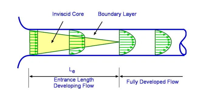
Hydrodynamic entrance length:
The hydrodynamic entrance region refers to the area of a pipe where fluid entering a pipe develops a velocity profile due to viscous
forces spreading from a pipe's interior wall. This region has a non-uniform flow. The fluid enters a pipe at a constant speed, so fluid
particles in the layer in contact with the pipe's surface come to a complete stop because of the no-slip rule. The layer in contact with
the pipe surface is resistant to the acceleration of neighboring layers due to viscous forces within the fluid and slowly slows down
adjacent layers of fluid, creating a velocity profile. To keep the mass true, the speed of the fluid layers in the center of the pipe
increases to compensate for the reduced speed of the fluid layers near the surface of the pipe. It creates a gradient of velocity across
the pipe cross-section.

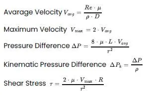
To do the simulation we need to find properties using some variables. Those are Hagen Poiseuille equations.
Variables :
Diameter ,D = 0.004
Radius, r = 0.002
Radial Distance, R = 0 to r
Dynamic viscosity, mu = 0.00089 N/m^2
Density, rho = 997 kg/m^3
Reyonlds number, Re =2100
Hagen poiseuille's Law:
In non ideal fluid dynamics, Hagen-poiseuille equation is a physical law that gives pressure drop in an incompressible and newtonian
fluid in a laminar flow through a long cylinder pipe of constant cross section.
Formulas:
Matlab Code:
clear all
close all
clc

% The Reynolds number
Re = 2100
% The Diameter of pipe
D = 0.004
% The Entry length of pipe
L =0.06*Re*D
% The total length of pipe
L_p = L+0.7
% Radius of pipe
r = D/2
% Angle of wedge (less than 5)
theta = 4
% Dynamic viscosity
mu = 0.89e-3
% Density
rho = 997

% Hagen poiseuille flow equations
v_avg = (Re*mu)/(rho*D)
v_max = 2*(v_avg)
del_p = (8*mu*L_p*v_avg)/(r^2)
kinematic_p = del_p/rho

% calculating shear stress
R = linspace(0,(D/2),1000)

for i = 1:length(R)
    tau(i) = 2*mu*v_max*(abs(R(i)))/r^2
end

plot(R,tau)
xlabel('Radius')
ylabel('Shear stress')
grid on
legend ('Shear stress')

header1='/*----------------------------------*- C++ -*------------------------------------*\'
header2='    =========                   | '
header3='    \\      /     F ield        | OpenFOAM: The Open Source CFD Toolbox '
header4='     \\    /      O peration    | Website: https://openfoam.org '
header5='      \\  /       A nd          | Version: 7 '
header6='       \\/        M anipulation | '
header7='\*---------------------------------------------------------------------------------*/'

f1 = fopen('blockMeshDict','w')
fprintf(f1, '%s\n', header1)
fprintf(f1, '%s\n', header2)
fprintf(f1, '%s\n', header3)
fprintf(f1, '%s\n', header4)
fprintf(f1, '%s\n', header5)
fprintf(f1, '%s\n', header6)
fprintf(f1, '%s\n', header7)

fprintf(f1, 'FoamFile\n{\n')
fprintf(f1, '%12s \t 2.0;\n','version')
fprintf(f1, '%12s \t ascii;\n','format')
fprintf(f1, '%12s \t dictionary;\n','class')
fprintf(f1, '%12s \t blockMeshDict;\n','object')
fprintf(f1, '}\n')
header8='// * * * * * * * * * * * * * * * * * * * * * * * * * * * * * * * * * * * * * //'
fprintf(f1, '%s\n\n',header8)


fprintf(f1, 'convertToMeters 1;\n\n')


fprintf(f1, 'vertices\n')
fprintf(f1, '(\n')
fprintf(f1, '\t (%d %d %d)\n',0,0,0)
fprintf(f1, '\t (%d %d %d)\n',0,r*cosd(theta/2),r*sind(theta/2))
fprintf(f1, '\t (%d %d %d)\n',0,r*cosd(theta/2),-r*sind(theta/2))
fprintf(f1, '\t (%d %d %d)\n',L_p,0,0)
fprintf(f1, '\t (%d %d %d)\n',L_p,r*cosd(theta/2),r*sind(theta/2))
fprintf(f1, '\t (%d %d %d)\n',L_p,r*cosd(theta/2),-r*sind(theta/2))
fprintf(f1, ');\n\n')


fprintf(f1, 'blocks\n')
fprintf(f1, '(\n')
fprintf(f1, '\t hex (0 3 5 2 0 3 4 1) (%d %d %d)',300,30,1)
fprintf(f1, ' SimpleGrading (1 0.1 1)\n\n')
fprintf(f1, ');\n\n')


fprintf(f1, 'edges\n')
fprintf(f1, '(\n')
fprintf(f1, '\t arc %d %d (%d %d %d)\n',1,2,0,r,0)
fprintf(f1, '\t arc %d %d (%d %d %d)\n',4,5,L_p,r,0)
fprintf(f1, ');\n\n')


fprintf(f1, 'boundary\n')
fprintf(f1, '(\n')
fprintf(f1, '\t inlet \n')
fprintf(f1, '\t {\n')
fprintf(f1, '\t\t type patch;\n')
fprintf(f1, '\t\t faces\n')
fprintf(f1, '\t\t (\n')
fprintf(f1, '\t\t\t (0 1 2 0)\n')
fprintf(f1, '\t\t );\n')
fprintf(f1, '\t }\n')


fprintf(f1, '\t outlet\n')
fprintf(f1, '\t {\n')
fprintf(f1, '\t\t type patch;\n')
fprintf(f1, '\t\t faces\n')
fprintf(f1, '\t\t (\n')
fprintf(f1, '\t\t\t (3 5 4 3)\n')
fprintf(f1, '\t\t );\n')
fprintf(f1, '\t }\n')


fprintf(f1, '\t top\n')
fprintf(f1, '\t {\n')
fprintf(f1, '\t\t type wall;\n')
fprintf(f1, '\t\t faces\n')
fprintf(f1, '\t\t (\n')
fprintf(f1, '\t\t\t (1 4 5 2)\n')
fprintf(f1, '\t\t );\n')
fprintf(f1, '\t }\n')


fprintf(f1, '\t front\n')
fprintf(f1, '\t {\n')
fprintf(f1, '\t\t type wedge;\n')
fprintf(f1, '\t\t faces\n')
fprintf(f1, '\t\t (\n')
fprintf(f1, '\t\t\t (0 3 4 1)\n')
fprintf(f1, '\t\t );\n')
fprintf(f1, '\t }\n')


fprintf(f1, '\t back\n')
fprintf(f1, '\t {\n')
fprintf(f1, '\t\t type wedge;\n')
fprintf(f1, '\t\t faces\n')
fprintf(f1, '\t\t (\n')
fprintf(f1, '\t\t\t (0 2 5 3)\n')
fprintf(f1, '\t\t );\n')
fprintf(f1, '\t }\n')

fprintf(f1, '\t axis\n')
fprintf(f1, '\t {\n')
fprintf(f1, '\t\t type empty;\n')
fprintf(f1, '\t\t faces\n')
fprintf(f1, '\t\t (\n')
fprintf(f1, '\t\t\t (0 3 3 0)\n')
fprintf(f1, '\t\t );\n')
fprintf(f1, '\t }\n')
fprintf(f1, '); \n\n')

fprintf(f1, 'mergePatchPairs\n')
fprintf(f1, '(\n')
fprintf(f1, ');\n')

header9='// * * * * * * * * * * * * * * * * * * * * * * * * * * * * * * * * * * * * *//'
fprintf(f1, '%s\n',header9)

fclose(f1)
BlockMeshDict:
/*--------------------------------*- C++ -*----------------------------------*\
   =========                    |
   \\      /      F ield        | OpenFOAM: The Open Source CFD Toolbox
    \\    /       O peration    | Website: https://openfoam.org
     \\  /        A nd          | Version: 7
      \\/         M anipulation |
\*---------------------------------------------------------------------------*/

FoamFile

{
   version        2.0;

   format         ascii;

   class          dictionary;

   object         blockMeshDict;
}

// * * * * * * * * * * * * * * * * * * * * * * * * * * * * * * * * * * * * * //

convertToMeters 1;

vertices

(

     (0 0 0)
     (0 1.998782e-03 6.979899e-05)
     (0 1.998782e-03 -6.979899e-05)
     (1.204000e+00 0 0)
     (1.204000e+00 1.998782e-03 6.979899e-05)
     (1.204000e+00 1.998782e-03 -6.979899e-05)

);

blocks

(

      hex (0 3 5 2 0 3 4 1) (300 30 1) SimpleGrading (1 0.1 1)

);

edges

(

     arc 1 2 (0 2.000000e-03 0)

     arc 4 5 (1.204000e+00 2.000000e-03 0)

);

boundary

(

     inlet

{

       type patch;

       faces

       (

              (0 1 2 0)

       );

}

     outlet

{

       type patch;

       faces

       (

          (3 5 4 3)

       );

}

     top

{

       type wall;

       faces

      (

         (1 4 5 2)

      );

}

    front

{

       type wedge;

       faces

      (

          (0 3 4 1)
      );

}

     back

{

       type wedge;

       faces

      (

         (0 2 5 3)

      );

}

    axis

{

      type empty;

      faces

     (

         (0 3 3 0)

     );

}

);

mergePatchPairs

(
);

// * * * * * * * * * * * * * * * * * * * * * * * * * * * * * * * * * * * * * //
ControlDict
/*--------------------------------*- C++ -*----------------------------------*\

    =========                  |
    \\      /    F ield        | OpenFOAM: The Open Source CFD Toolbox
     \\    /     O peration    | Website: https://openfoam.org
      \\  /      A nd          | Version: 7
       \\/       M anipulation |

\*---------------------------------------------------------------------------*/

FoamFile

{
  version     2.0;

  format      ascii;

  class       dictionary;

  location    "system";

  object      controlDict;

}

// * * * * * * * * * * * * * * * * * * * * * * * * * * * * * * * * * * * * * //

application          icoFoam;

startFrom            startTime;

startTime            0;

stopAt               endTime;

endTime              1;

deltaT               0.001;

writeControl         timeStep;

writeInterval        20;

purgeWrite           0;

writeFormat          ascii;

writePrecision       6;

writeCompression     off;

timeFormat           general;

timePrecision        6;

runTimeModifiable    true;


// ************************************************************************* //
Velocity Boundary Condition:
/*--------------------------------*- C++ -*----------------------------------*\

   =========                   |
   \\      /     F ield        | OpenFOAM: The Open Source CFD Toolbox
    \\    /      O peration    | Website: https://openfoam.org
     \\  /       A nd          | Version: 7
      \\/        M anipulation |

\*---------------------------------------------------------------------------*/

FoamFile

{

   version      2.0;

   format       ascii;

   class        volVectorField;

   object       U;

}

// * * * * * * * * * * * * * * * * * * * * * * * * * * * * * * * * * * * * * //

dimensions          [0 1 -1 0 0 0 0];

internalField       uniform (0.4686 0 0);

boundaryField

{

   inlet

  {

     type         fixedValue;

     value        uniform (0.4686 0 0);

  }

   outlet

  {

     type         zeroGradient;

  }

   axis

  {

     type         empty;

  }

   top

  {

     type         fixedValue;

     value        uniform (0 0 0);

  }

   front

  {

     type         wedge;

  }

   back

  {

     type         wedge;

  }

}

// ************************************************************************* //
Pressure Boundary Condition:
/*--------------------------------*- C++ -*----------------------------------*\

  =========                    |
  \\      /      F ield        | OpenFOAM: The Open Source CFD Toolbox
   \\    /       O peration    | Website: https://openfoam.org
    \\  /        A nd          | Version: 7
     \\/         M anipulation |

\*---------------------------------------------------------------------------*/

FoamFile

{

  version   2.0;

  format    ascii;

  class     volScalarField;

  object    p;

}

// * * * * * * * * * * * * * * * * * * * * * * * * * * * * * * * * * * * * * //

dimensions      [0 2 -2 0 0 0 0];

internalField   uniform 0;

boundaryField

{

   inlet

  {

      type       zeroGradient;

  }

   outlet

  {

      type       fixedValue;

      value      uniform 1.0073;

  }

   axis

  {

      type       empty;

  }

   top

  {

     type        zeroGradient;

  }

   front

  {

     type        wedge;

  }

   back

  {

     type        wedge;

  }

}

// ************************************************************************* //
Transport properties
/*--------------------------------*- C++ -*----------------------------------*\

  =========                  |
  \\      /    F ield        | OpenFOAM: The Open Source CFD Toolbox
   \\    /     O peration    | Website: https://openfoam.org
    \\  /      A nd          | Version: 7
     \\/       M anipulation |

\*---------------------------------------------------------------------------*/

FoamFile

{

  version     2.0;

  format      ascii;

  class       dictionary;

  location    "constant";

  object      transportProperties;

}

// * * * * * * * * * * * * * * * * * * * * * * * * * * * * * * * * * * * * * //

nu            [0 2 -1 0 0 0 0] 8.9256e-07;

// ************************************************************************* //
Results:
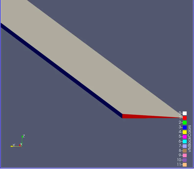
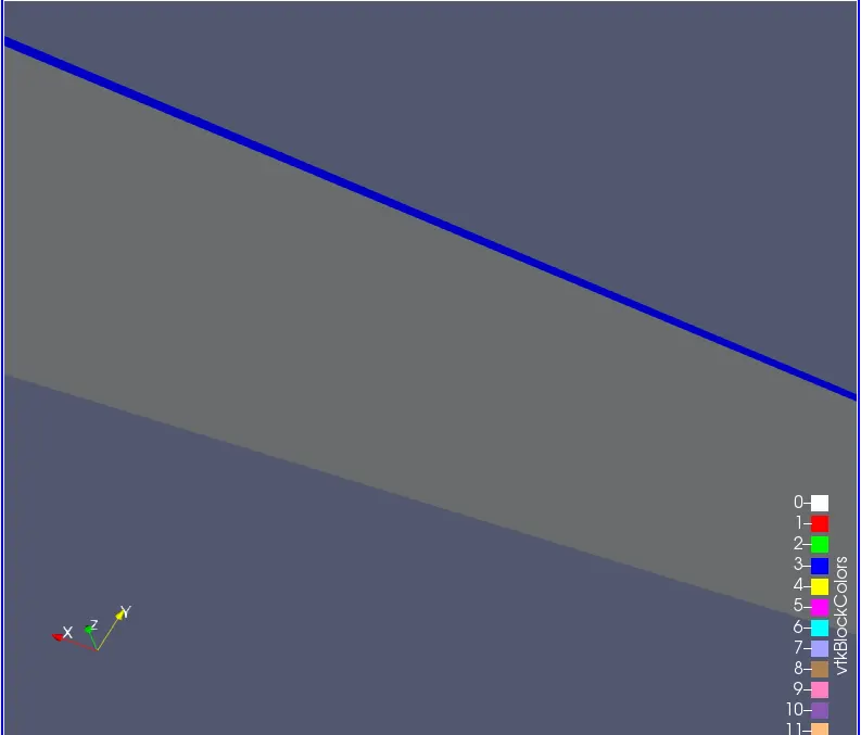
Generated Gometry and Mesh:
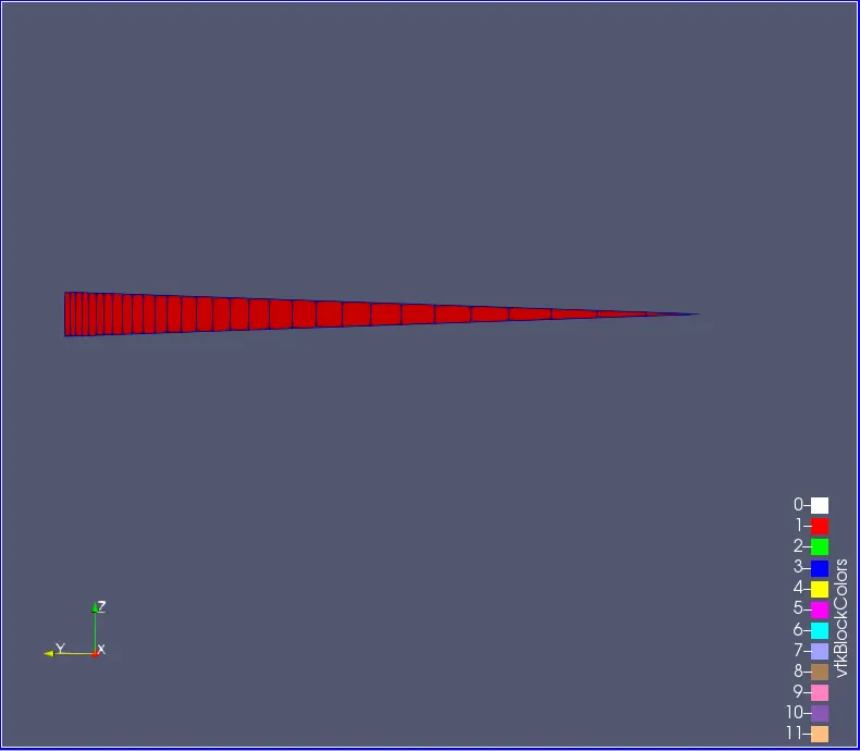
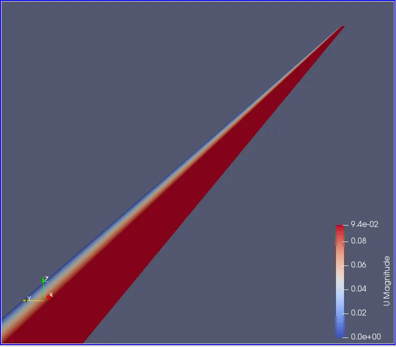
Post Processing:
- After opening paraview click on generate to see the geometry. View the geometry from different sides across X,Y and Z axes.
- Press on the play button to post process to end time.
- Click on filters and select plot over line and plot velocity magnitude and pressure with respect to radial distance.
- Export the velocity data in .csv format.
- For calculating the shear stress import the .csv file into MATLAB/Octave.
- Select the suitable column to plot shear stress.
- Write a MATLAB/Octave code to calculate shear stress.
- The shear stress should be maximum at walls.
- Plot the result for shear stress.
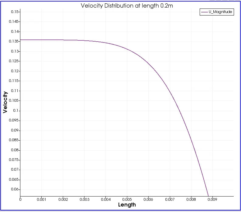
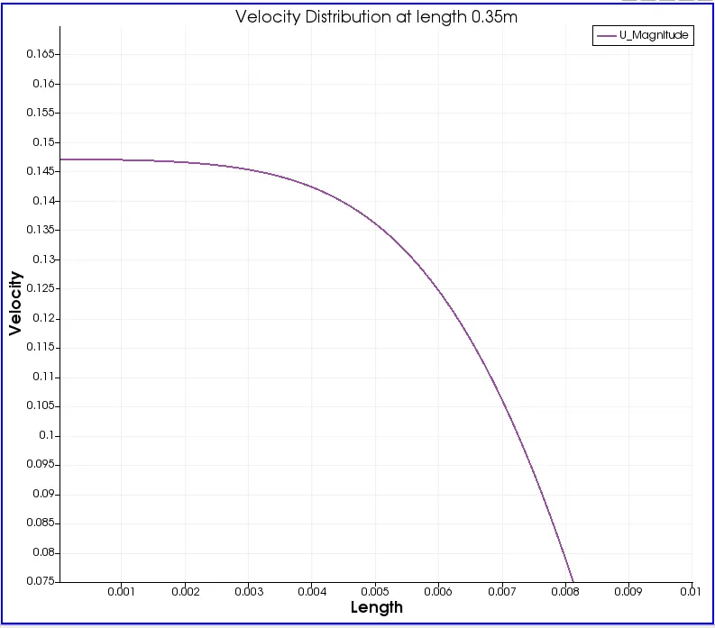
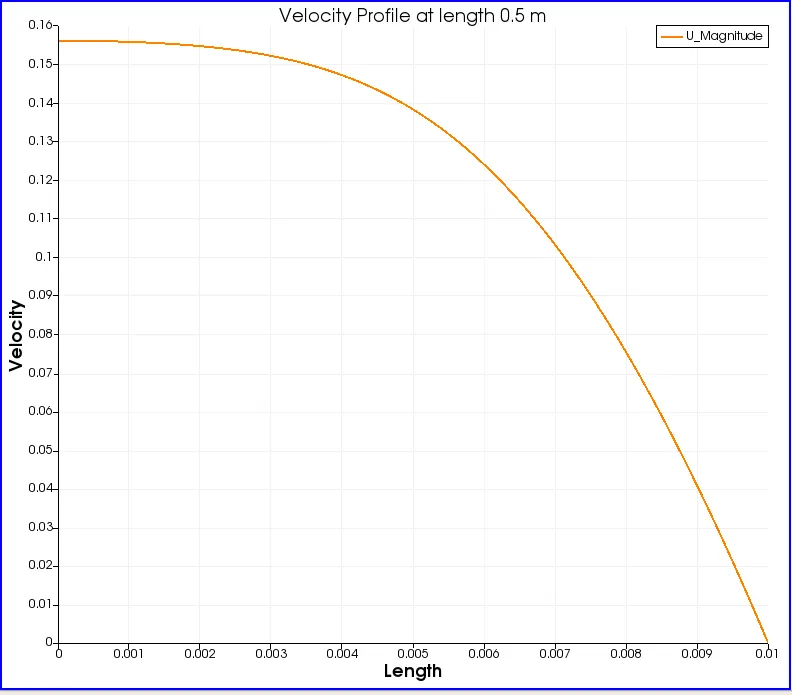
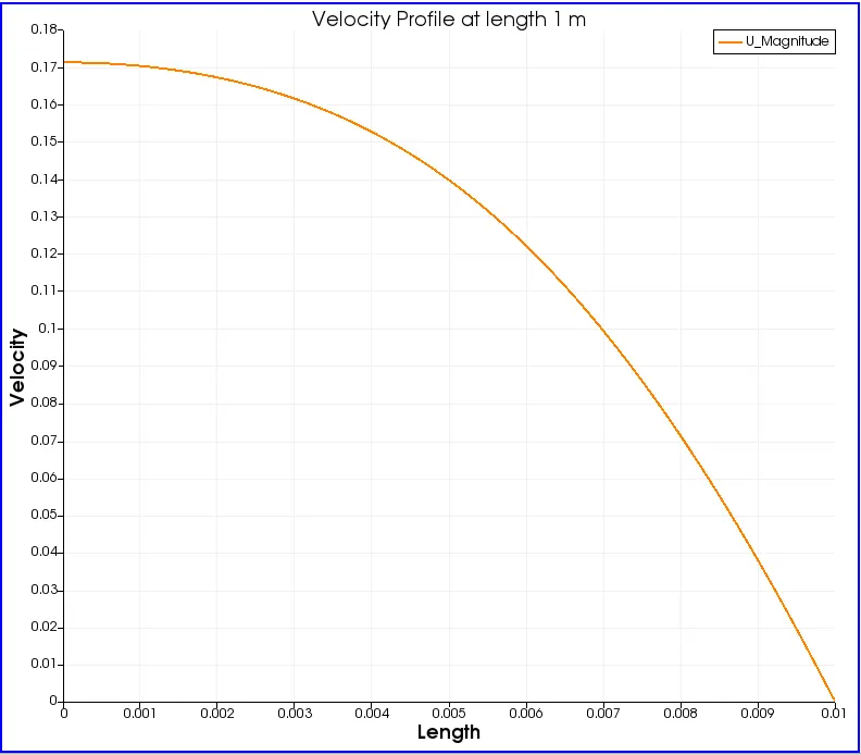
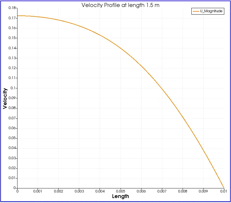
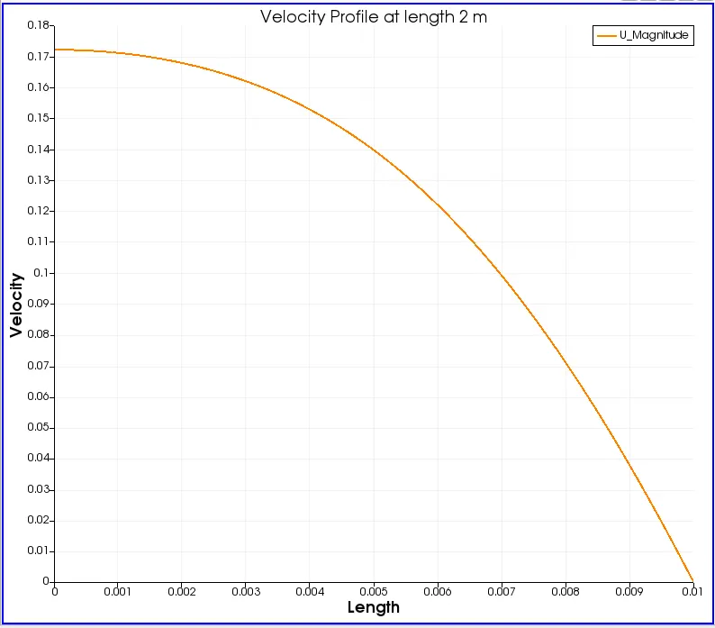
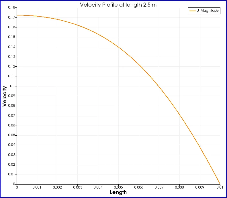
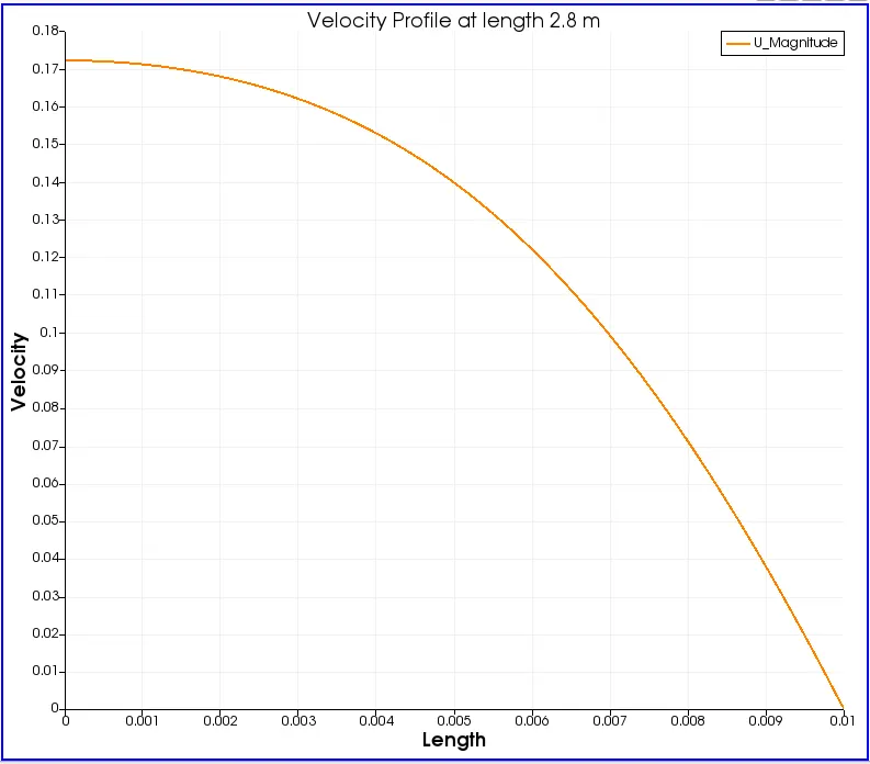
Velocity Profiles(Graphical Representation)
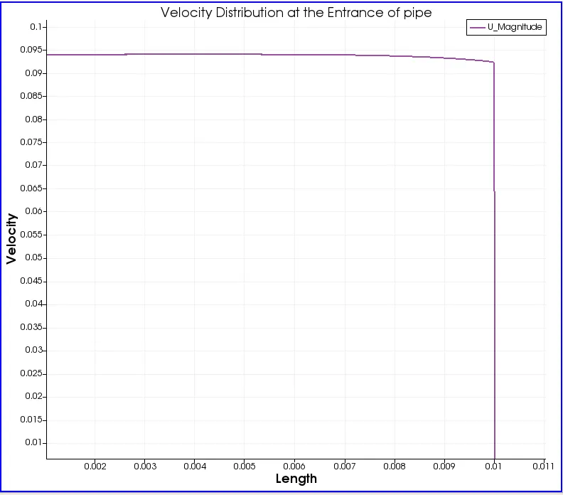
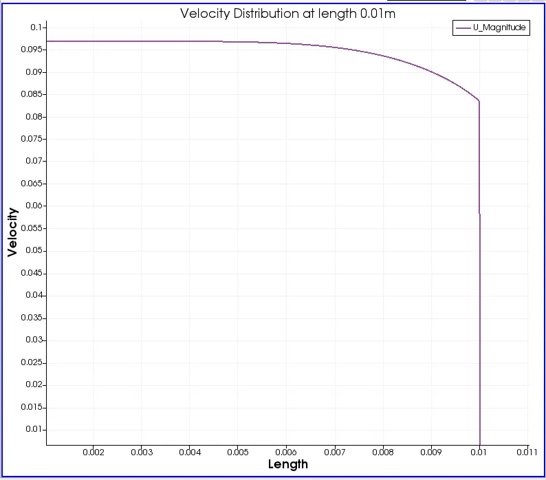
1.
2.
3.
4.
5.
6.
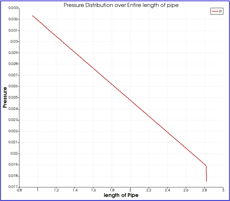
Pressure Profile (Graphical Representation)
Calculating shear stress:
clear all
close all
clc

D = 0.02
R = D/2
r = linspace(-0.01,0.01,1000)
Re = 2100
mu = 8.9e-4
rho = 997.130
V = (Re*mu)/(rho*D)
u_max = 2*V

for i= 1:length(r)
    Tau(i) = (2*mu*u_max*abs(r(i)))/(R^2);
end

figure(1)
plot(r,Tau)
xlabel('Radial Distance in m')
ylabel('Shear Stress(Tau) in N/m^2')
title(sprintf('change in shear stress for fully developed flow at x=2.82m with radial distance'))
grid minor

u=csvread('velocity.csv','A2:A1002');
y = linspace(-0.005,0.005,1000);
dy = y(2)-y(1);

for k=336:length(y);
    du(k)=u(k+1)-u(k);
    tau(k)=mu*(abs(du(k))/dy);
end

figure(2)
plot(r,tau)
xlabel('Radial Distance in m')
ylabel('Shear Stress(tau) in N/m^2')
title(sprintf('change in shear stress for fully developed flow at x=2.82m with radial distance'))
grid minor
Result
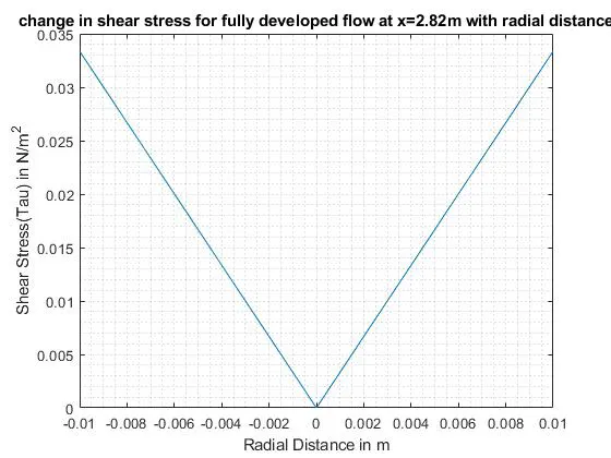
not equal to zero because it is calculated at 1m length in which the flow is not fully developed so it is not equal to zero.
Shear stress:
- When the fluid is in motion, shear stresses are developed due to the particles in the fluid moving relative to one another.
- For a fluid flowing in a pipe Fluid velocity will be zero at the pipe wall. Velocity will increase while moving towards the center of the
pipe. Shear Force is normally present because the adjacent layer of the fluid move with different velocities compared to each other. - Fluids Obeying Newton's law where the values of “mu” are constant are known as Newtonian fluids. If ‘mu’ is constant, the shear
stress is linearly dependent on the velocity gradient.
By considering the velocity of this relative motion, the Shear rate can be calculated shear rate is defined as a measurement of the
extent or rate of relative motion between the adjacent layer of the moving fluid. The shear rate for fluid flowing between two parallel
plates one moving at a constant speed and one is stationary.
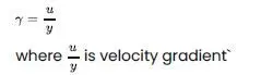
shear stress is propotional to the shear rate where viscosity is the propotionality cofficient.
this is known as Newtons's law of viscocity
tau = mu((du)/(dy))`
1. The above expression is valid only for the low range of Reynolds numbers like laminar flows.
2. coming to the turbulent flows it doesn’t work because are any well-defined layers. Instead, unsteady vortices appear of many
sizes that interact with each other in a rather chaotic manner
3. A separate code has to write to calculate the shear stress numerically.
4. Before that, we need to extract the velocity values from the OpenFOAM.
5. Using a “CSV” file, we can extract all the velocity (U_magnitude, U_x, U_y, U_z) and pressure values. The “.CSV” is more like an
Excel sheet, directly we can upload it to Matlab.
6. After uploading it into Matlab, Select only “u” (U_magnitude) values and upload it to the workspace.
7. After uploading we need to write a Matlab code to calculate the shear stress.
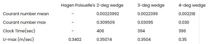
The above table shows that the max velocity of simulation is equal to the hagen poisuelle's velocity.
The change in wedge angle(wedge angle<5)does'nt affect the result of simulation. For wedge angle 2 3 and 4 the solution is same.