Week 7 - Simulation of a 1D Super-sonic nozzle flow simulation using Macormack Method

PROJECT-

-To stimulate the isentropic Flow through a quasi 1D subsonic-supersonic nozzel using Matlab.

OBJECTIVES-

• Derive both the conservation and non-conservation forms of the governing equations and sovle them using the MacCormack's technique.
• Determine the steady-state temperature distribution for the flow-field variables and investigate the difference between the conservation and non-conservation forms of governing equations .
• Comparison of Normalized mass flow rate distributions of both conservation and non-conservation forms and check which metod is faster .

THEORY-

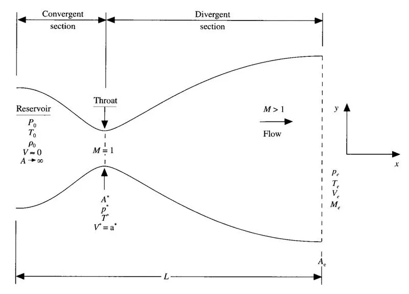
1D SUPERSONIC NOZZEL FLOW is devided into three part ,the convergent part which conected into the resevoir. It is also called as subsonic flow through nozzel and the mach no. in this area is lees than 1. : Mach number<1.

In the throat mach number is equal to 1 ,that means the sound of speed is equal to fluid speed. :Mach number =1.

In divergent also called as supersonic condition the mach number is greater than 1,fluid speed is maximum in divegent and velocity of fluid is more than that of speed of sound. : Mach number>1

QUASI 1D FLOW-

- The area of sonic throat is denoted by *A, and We assume that at a given section ,where the cross sectional area is A the floew properties are uniform across that section hence the area of nozzel changes as a function of distance along the the nozzel, in reality the flow field is two dimensional but we make the assumption that the flow properties vary only with x,this is the tantamount to assuming uniform flow properties across any given cross section . such flow is defiend as Quasi 1D flow.

- Difference between one-dimenstional and quasi one -dimenstional flow,

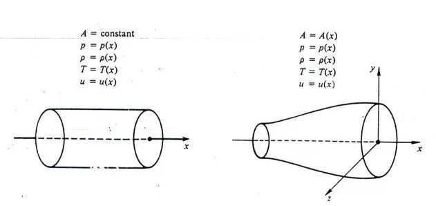
(One Dimenstional) (Quasi one Dimensional)

GOVERNING EQUATION

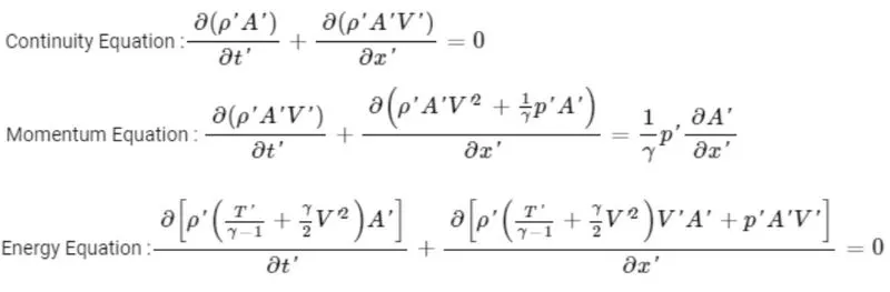
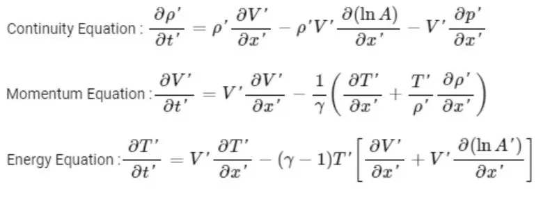
-The super sonic flow through nozzel is governed by navier stroke equations ,which can be written for both conservative and non-conservative forms.

• Conservative equations:-

• Non-conservatve equation:-

MACCORMACK METHOD-

-We chose this method to illustrate both explicit and implicit finite difference method which is second order accurate, both in space and time. In paticular we will set up time marching finite diference solution for quasi 1D nozzel flow

MAIN PROGRAM-

-For conservation and Non conservation form

clear alll
close all 
clc
%Solving Quasi 1d supersonic nozzle flow equation
%inputs
n = 31;

gamma = 1.4;
C=0.5;
x = linspace(0,3,n);
dx = x(2)-x(1);
nt = 1400;
th = (n-1)/2;
t_array = 1:1400;
A = 1+(2.2*((x-1.5).^2));

%Function for non conservative form
tic;
[m,M,v,T,p,rho,T_th,rho_th,p_th,M_th]= Non_conservative(x,dx,n,C,A,nt,gamma,th)
Time_elapsed = toc;
fprintf('Time Elasped of properties at throat area in non conservative form=%0.4f',Time_elapsed)


%ploating
%Time steps variation of properties area in non conservative form
figure(2)

%Density
subplot(4,1,1)
plot(t_array,rho_th,'r')
ylabel('Density')
legend({'Density at throat'})
axis([0 1400 0 1])
grid minor
title('timestep variation at throat area -Non conservative form')

%Temperature
subplot(4,1,2)
plot(t_array,T_th,'b')
ylabel('Temperature')
legend({'Temperatureat throat'})
axis([0 1400 0.6 1])
grid minor

%Presure
subplot(4,1,3)
plot(t_array,p_th,'g')
ylabel('Presure')
legend({'Presure at throat'})
axis([0 1400 0 1.5])
grid minor

%Mach Number
subplot(4,1,4)
plot(t_array,M_th,'m')
xlabel('Timesteps')
ylabel('Mach number')
legend({'Mach number at throat'})
axis([0 1400 0.6 2])
grid minor

%Steady state stimulation for primitive values for Non conservative form
figure(3)
%Density
subplot(4,1,1)
plot(x,rho,'-r')
ylabel('density')
legend('density')
grid minor
title('Variation of flow rate distribution-Non conservative')

%Temprature
subplot(4,1,2)
plot(x,T,'-b')
ylabel('Temprature')
legend('Temprature')
grid minor

%Presure
subplot(4,1,3)
plot(x,p,'-g')
ylabel('Presure')
legend('Presure')
grid minor

%Mach number
subplot(4,1,4)
plot(x,M,'-m')
ylabel('Mach Number')
legend('Mach number')
grid minor

%Function for conservative form
tic;
[m_c,M_c,v_c,T_c,p_c,rho_c,T_th_c,rho_th_c,p_th_c,M_th_c]= Conservative(x,dx,n,C,A,nt,gamma);
Time_elapsed = toc;
fprintf('Time Elasped of properties at throat area in conservative form: 0.4f',Time_elapsed);

%ploating
%Time steps variation of properties area in conservative form
figure(5)

%Density
subplot(4,1,1)
plot(t_array,rho_th_c,'b')
ylabel('Density')
legend({'Density at throat'})
axis([0 1400 0 1.3])
grid minor
title('timestep variation at throat area -Conservative form')

%Temperature
subplot(4,1,2)
plot(t_array,T_th_c,'r')
ylabel('Temperature')
legend({'Temperatureat throat'})
axis([0 1400 0 1.5])
grid minor

%Presure
subplot(4,1,3)
plot(t_array,p_th_c,'g')
ylabel('Presure')
legend({'Presure at throat'})
axis([0 1400 0 1.5])
grid minor

%Mach Number
subplot(4,1,4)
plot(t_array,M_th_c,'m')
xlabel('Timesteps')
ylabel('Mach number')
legend({'Mach number at throat'})
axis([0 1400 0.1 1.8])
grid minor

%Steady state stimulation for primitive values for Non conservative form
figure(6)
%Density
subplot(4,1,1)
plot(x,rho_c,'-b')
ylabel('density')
legend('density')
grid minor
title('Variation of flow rate distribution- Conservative')

%Temprature
subplot(4,1,2)
plot(x,T_c,'-r')
ylabel('Temprature')
legend('Temprature')
grid minor

%Presure
subplot(4,1,3)
plot(x,p_c,'-g')
ylabel('Presure')
legend('Presure')
grid minor

%Mach number
subplot(4,1,4)
plot(x,M_c,'-m')
ylabel('Mach Number')
legend('Mach number')
grid minor

%Comparision pkot of normalized masss flow rate of both forms
figure(7)
hold on 
plot(x,m,'r',LineWidth=1.5)
plot(x,m_c,'b','LineWidth',1.5)
line([0 3],[0.579 0.579],'linewidth',1.5)
grid minor 

legend('Non conservative ','Conservative')
xlabel('Length of the domain')
ylabel('Mass flow rate')
title('Comaparison of noarmalized mass flow rate of both forms')

FUNCTION FOR NON CONSERVATIVE FORM-

%function for non conservative form

function [m,M,v,T,p,rho,T_th,rho_th,p_th,M_th]= Non_conservative(x,dx,n,C,A,nt,gamma,th);

%Intial boundary condition
rho_initial = 1-(0.3146*x);
T_initial = 1-(0.2341*x);
v_initial = (0.1+(1.09*x)).*(T_initial.^0.5);

%Area & Throat profiles
A = 1+(2.2*((x-1.5).^2))
%%field variables
rho = rho_initial
T = T_initial
v = v_initial
p = rho.*T;
M = v./(T.^0.5)
m = rho.*v.*A;
%%Stencil metrics for throat section
th = find(A==1); 

%time steps
for i = 1:n
    dt_cl(i) = (0.5*dx)/((T(i)).^0.5 +v(i));
end
dt = min(dt_cl)
%No of timesteps
nt = 1400


%Outer time loop
for k = 1:nt

    %Saving old values
    rho_old = rho;
    T_old = T;
    v_old = v;
    p_old = p;
    M_old = M;


    %Predictor method
    for i = 2:n-1

        %Simplifying the euation in spatia term
        drho_dx = (rho(i+1)-rho(i))/dx;
        dv_dx = (v(i+1)- v(i))/dx;
        dT_dx = (T(i+1) - T(i))/dx;
        dlog_a_dx = (log(A(i+1))-log(A(i)))/dx;

        %Continutiy Equation
        drho_dt_p(i) = -rho(i)*dv_dx - rho(i)*v(i)*dlog_a_dx-v(i)*drho_dx;

        %Momentum equation
        dv_dt_p(i)= -v(i)*dv_dx-(1/gamma)*(dT_dx+(T(i)*drho_dx/rho(i)));

        %Energy equation
        dT_dt_p(i) = - v(i)*dT_dx-(gamma-1)*T(i)*(dv_dx + v(i)*dlog_a_dx);

        %Solution updaate
        rho(i) = rho(i) + drho_dt_p(i)*dt;
        v(i) = v(i) + dv_dt_p(i)*dt;
        T(i) = T(i) + dT_dt_p(i)*dt;

    end

    %Corrector Method
    for i = 2:n-1

        %Simplifying the euation in spatia term
        dv_dx = (v(i)-v(i-1))/dx;
        drho_dx = (rho(i)- rho(i-1))/dx;
        dT_dx = (T(i) - T(i-1))/dx;
        dlog_a_dx = (log(A(i))-log(A(i-1)))/dx;

        %Continutiy Equation
        drho_dt_c(i) = -rho(i)*dv_dx - rho(i)*v(i)*dlog_a_dx-v(i)*drho_dx;

        %Momentum equation
        dv_dt_c(i)=-v(i)*dv_dx-(1/gamma)*(dT_dx+(T(i)*drho_dx/rho(i)));

        %Energy equation
        dT_dt_c(i) = - v(i)*dT_dx-(gamma-1)*T(i)*(dv_dx + v(i)*dlog_a_dx);

    end

        %Compute average time derivative
        drho_dt_avg = 0.5.*(drho_dt_p + drho_dt_c);
        dv_dt_avg =  0.5.*(dv_dt_p + dv_dt_c);
        dT_dt_avg =  0.5.*(dT_dt_p + dT_dt_c);
    
        %Final solution update 
        for j = 2:n-1
        rho(j) = rho_old(j)+drho_dt_avg(j)*dt
        v(j) = v_old(j)+dv_dt_avg(j)*dt;
        T(j) = T_old(j)+dT_dt_avg(j)*dt;
    end

    %Applyinf boundary condition
    %At inlet
    v(1) = 2*v(2)-v(3)
    
    
    %at outlet
    rho(n) = 2*rho(n-1) - rho(n-2);
    v(n) = 2*v(n-1)-v(n-2)
    T(n) = 2*T(n-1)-T(n-2)

    %Defining mass flow rate , pressure and mach number
    m = rho.*v.*A
    p = rho.*T
    M = (v./(T.^0.5))
    
    %calculating variable at throat section 
    rho_th(k)  = rho(th);
    T_th(k) = T(th);
    v_th(k) = v(th)
    p_th(k) = p(th);
    M_th(k) = M(th);

    %ploating
    %comparison of non dimensional mass flow rates at different time steps
    figure(1)
    hold on
    if k == 50
        plot(x,m,'r','linewidth',1.5)
    else if k ==100
            plot(x,m,'b','linewidth',1.5)
    else if k == 200
            plot(x,m,'g','linewidth',1.5)
    else if k ==4
            plot(x,m,'m','linewidth',1.5)
    else if k == 700
            plot(x,m,'-','linewidth',1.5)
            plot(x(end),m(end),'b*')
    end
    end
    end
    end
    end
    %labelling
    title('Mass flow rate at different timesteps - Non conservative form')
    xlabel('Distance')
    ylabel('Mass flow rate')
    legend({'50^t^h timestep','100^t^h timestep','200^t^h timestep','400^t^h timestep','500^t^h timestep'})
    axis([0 3 0 2.5])
    grid on
    grid minor
end
       

EXPLANATIION FOR NON CONSEVATIVE EQUATION-

-First we take initial conditions as follow as,

• `A = 1+2.2(x-1.5)^2`
• `rho = 1-0.3146x`
• `T = 1-0.2314x`
• `V = (0.1+1.09)^(T)overset(1/2)`

-The nozzel shape A= a(x) is specified and held fixed independent of time ,for the case illustration is this section we choose a parabolic area distribution.

-`The density temperature and velocity is given above(Initial condition at t=o)`.

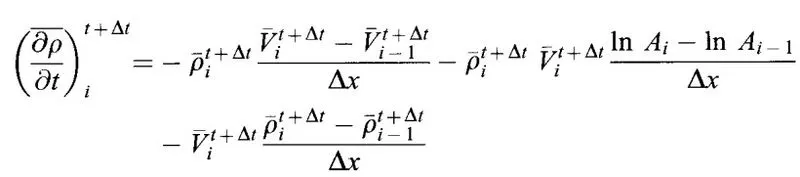
- Then we take predictor step a provisional value of u at time level `n+1`is esimated obtained by repalcing the spatial and temporal derivatives in the previous first order equation using forward difference scheme .

`((delrho)/(delt))overset(t)underset(i,j)``= -(rhooverset(t)underset(i,j)``(uoverset(t)underset(i+1,j) -uoverset(t)underset(i,j))/(Deltax)``+uoversettunderset(i,j)``(rhooversettunderset(i+1,j) -rho oversettunderset(i,j))/(Deltax)+rhooversettunderset(i,j)``(voversettunderset(i+1,j)-voversett(underset)(i,j))/(Deltay)-vunderset(i,j)``rhooversettunderset(i+1,j) -(rhooversettunderset(i,j))/(Deltay)`

- In above equation all flow variables at time t are known predcted value from taylor series.

-Corrector step is for predict the value `(u)undersetioverset(n+1)` is corrected according to the equation .The corrector step uses bacward difference scheme for special derivative.The time steps used in the corrector step is `(Deltat)/2`in constant to the `Deltat` used in the predictor step.

-Average Value

`((delrho)/(dt))underset(avg)``1/2[((delrho)/(delt))underset(i,j)overset(t)``+(overline((delrho)/(delt)))overset(t+Deltat)underset(i,j)`

-Boundary condition-

Inflow boundary condition:

`Vunderset1 =2Vunderset2-Vunderset3`

Outflow boundary condition:

`VundersetN = 2Vunderset(N-1) - V(N-2)`

`TundersetN = 2Tunderset(N-1) - Tunderset(N-2)`

`rhoundersetN = 2rhounderset(N-1)+rhounderset(N-2)`

RESULT-

For non conservative form (n-31grid point)

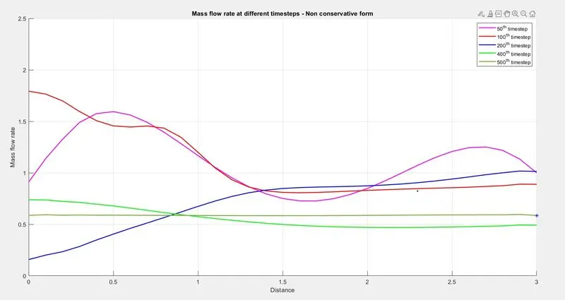
(mass flow rate of different time steps)

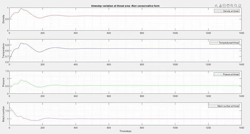
-Time step variation of primitive variable at throat area(Non_conservative)

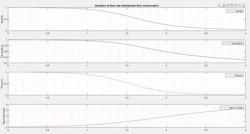
-Variattion of flow rate distribution(Non_conservative)

FUNCTION CODE FOR CONSERVATION FORM-

%function for non conservative form

function [m_c,M_c,v_c,T_c,p_c,rho_c,T_th_c,rho_th_c,p_th_c,M_th_c]= Conservative(x,dx,n,C,A,nt,gamma)
%Intial profile of density and temprature
for i = 1:length(x)
    if  x(i)>=0 && x(i) <=0.5
        rho_c(i) = 1.0;
        T_c(i) = 1.0;
    else if x(i)>= 0.5 && x(i) <=1.5
        rho_c(i) = 1-0.366*(x(i) - 0.5);
        T_c(i) = 1-0.167*(x(i)-0.5);
    else if x(i) >= 1.5 && x(i) <= 3.0;
        rho_c(i) = 0.634-0.3879*(x(i) - 1.5);
        T_c(i) = 0.833 - 0.3507*(x(i)-1.5);
    end
    end
    end
end
   

%Area and throat profiles
A = 1 +(2.2*((x - 1.5).^2));

%initial profile for velocity and pressure
v_c = 0.59./(rho_c.*A)
p_c = rho_c.*T_c;
m_c = rho_c.*A.*v_c;
M_c = v_c./(T_c.^0.5);

%Non dimenstional flow field variables at throat
th = find(A==1);
rho_th_c = rho_c(th);
T_th_c = T_c(th);
v_th_c = v_c(th);
p_th_c = p_c(th);
M_th_c = M_c(th);
m_th_c = m_c(th);

%Timesteps
CFL = 0.5;
for i = 1:n
    dt_c_cal(i) = (CFL.*dx)/(((T_c(i)).^0.5)+v_c(i));
end
dt_c = min(dt_c_cal);
%calculate the initial solution vector (U)
U1 = rho_c.*A;
U2 = rho_c.*A.*v_c;
U3 = rho_c.*A.*(T_c./(gamma - 1) +(gamma./2).*v_c.^2);
nt = 1400;

%Outer time loop
for k = 1:nt

    %Calculating the flux vector(F)
    F1 = U2;
    F2 = ((U2.^2)./U1) + ((gamma-1)./gamma).*(U3- (gamma./2).*((U2).^2./U1));
    F3 = ((gamma.*U2.*U3)./U1)-((gamma.*(gamma-1))./2).*((U2.^3)./(U1.^2));
    
    %Saving old values
    U1_old = U1
    U2_old = U2
    U3_old = U3

    %Predictor method
    for i = 2:n-1

        %calculating the source term(j)
        J2(i) = (1/gamma)*rho_c(i)*T_c(i)*((A(i+1)- A(i))/dx)

        %Continutiy Equation
        dU1_dt_p(i) = -((F1(i+1) - F1(i))./dx);

        %Momentum equation
        dU2_dt_p(i)=-((F2(i+1) - F2(i))./dx) +J2(i);

        %Energy equation
        dU3_dt_p(i) = -(F3(i+1) - F3(i))./dx;

        %Uodating new variable
        U1(i) = U1_old(i) + dU1_dt_p(i).*dt_c;
        U2(i) = U2_old(i) + dU2_dt_p(i).*dt_c;
        U3(i) = U3_old(i) + dU3_dt_p(i).*dt_c;
        %premitative variable from solution vector
        rho_c(i) = U1(i)./A(i);
        v_c(i) = (U2(i)./U1(i));
        T_c(i) = (gamma-1).*((U3(i)./U1(i))-(gamma./2).*((U2(i)./U1(i)).^2))
        p_c(i) = rho_c(i).*T_c(i);
    end
    %Updating Flux vector
    F1 = U2;
    F2 = ((U2.^2)./U1) + ((gamma-1)./gamma).*(U3- (gamma./2)*((U2).^2./U1));
    F3 = ((gamma.*U2.*U3)./U1)-((gamma.*(gamma-1))./2).*((U2.^3)./(U1.^2));

    

    %Corrector Method
    for i = 2:n-1
        
        %Upating the source term(3)
        J2(i) = (1/gamma)*rho_c(i)*T_c(i)*((A(i)- A(i-1))/dx)

        %Simplifying the euation in spatia term
        dU1_dt_c(i) = -((F1(i)-F1(i-1))./dx);
        dU2_dt_c(i) = -((F2(i)-F2(i-1))./dx)+J2(i);
        dU3_dt_c(i) = -((F3(i) - F3(i-1))./dx);
        
    end

    %Compute average time derivative
    dU1_dt_avg =  0.5.*(dU1_dt_p + dU1_dt_c);
    dU2_dt_avg =  0.5.*(dU2_dt_p + dU2_dt_c);
    dU3_dt_avg =  0.5.*(dU3_dt_p + dU3_dt_c);
    
    %Final solution update
    for j = 2:n-1
        U1(j) = U1_old(j)+dU1_dt_avg(j).*dt_c
        U2(j) = U2_old(j)+dU2_dt_avg(j).*dt_c;
        U3(j) = U3_old(j)+dU3_dt_avg(j).*dt_c;
    end

    %Applyinf boundary condition
    %At inlet
    U1(1) = rho_c(1)*A(1);
    U2(1) = 2*U2(2)-U2(3);
    U3(1) = U1(1)*((T_c(1)/(gamma-1)) +((0.5*gamma)*(v_c(1)).^2))
    
    %at outlet
    U1(n) = 2*U1(n-1) - U1(n-2);
    U2(n) = 2*U2(n-1) - U2(n-2)
    U3(n) = 2*U3(n-1) - U3(n-2)

    %Final primitative value update
    rho_c = U1./A;
    v_c = U2./U1;
    T_c = (gamma - 1).*((U3./U1)-(gamma./2).*((U2./U1).^2));
    p_c = rho_c.*T_c;
    m_c = rho_c.*A.*v_c;
    M_c = v_c./(sqrt(T_c));
    
    %calculating variable at throat section 
    rho_th_c(k)  = rho_c(th);
    T_th_c(k) = T_c(th);
    v_th_c(k) = v_c(th);
    m_th_c(k) = m_c(th);
    p_th_c(k) = p_c(th);
    M_th_c(k) = M_c(th);

    %ploating
    %comparison of non dimensional mass flow rates at different time steps
    figure(4)
    hold on
    if k == 100
        plot(x,m_c,'b','linewidth',1.5)
    else if k == 200
        plot(x,m_c,'r','linewidth',1.5)
    else if k == 400
        plot(x,m_c,'g','linewidth',1.5)
    else if k == 700
        plot(x,m_c,'o','linewidth',1.5)
    end
    end
    end
    end
    %labelling
    title('Mass flow rate at different timesteps - conservative form')
    xlabel('Distance')
    ylabel('Mass flow rate')
    legend('100^t^h timestep','200^t^h timestep','400^t^h timestep','700^t^h timestep')
    axis([0 3 0.4 1.5])
    grid on
    grid minor
end
     

EXPLANATION FOR CONSERVATION FORM EQUATION-

conserve from complex into a simpler form

`(delU1)/(delt') = -(delF1)/(delx')`

`(delU2)/(delt') = -(delF2)/(dx')+J2`

`(delU3)/(delt')=-(delF3)/(delx')`

-Flux term and source term in form solution vector

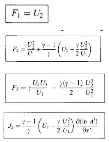
where U is the solutiom vector ,F is flux vector and J2 is source term

-Initial condition

• For `0lex'le0.5`

`rho' = 1.0`

`T'=1.0`

• For `0.5lex'le1.5`

`rho' = 1-0.366(x'-0.5)`

`T' = 1-0.167(x'-0.5)`

• For `1.5lex'le3.5`

`rho' = 0.634-0.3879(x'-1.5)`

`T' = 0.833-0.3507(x'-1.5)`

-Boundaary condition

• Inlet boundary conditions

`Uunderset(1(i=1)``=(rho'A')underset(i=1) =A'underset(i=1)`

`Uunderset(2(i-1)``=2Uunderset(2(i=2))-Uunderset(2(i-3)`

`Uunderset(3)=rho'((e')/(gamma-1)+(gamma)/2*V'^2)A'`

• Outlet boundary conditions

`(U1)undersetN``= 2(U1)underset(N-1)-(U1)underset(N-2)`

`(U2)undersetN` `=2(U2)underset(N-1)-(U2)underset(N-2)`

`(U3)undersetN``=2(U3)underset(N-1)-(U3)underset(N-2)`

RESULT-

For conservative form (n-31grid point)

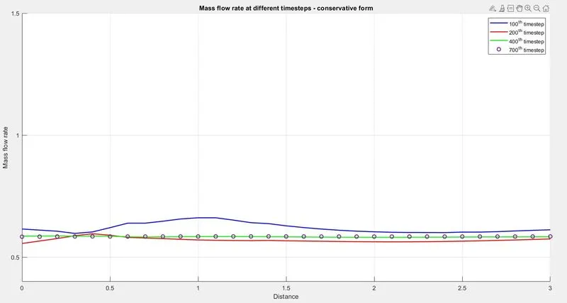
(mass flow rate of different time steps)

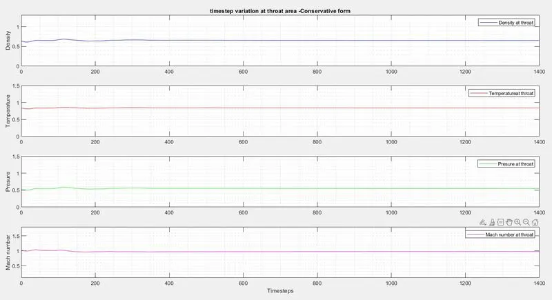
-Time step variation of primitive variable at throat area(Conservative)

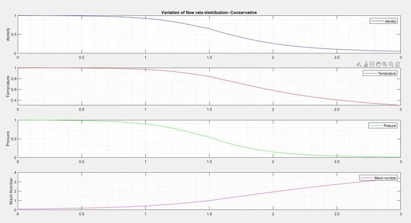
-Variattion of flow rate distribution(Conservative)

-Comparison of mass flow rate of non conservative and conservative form

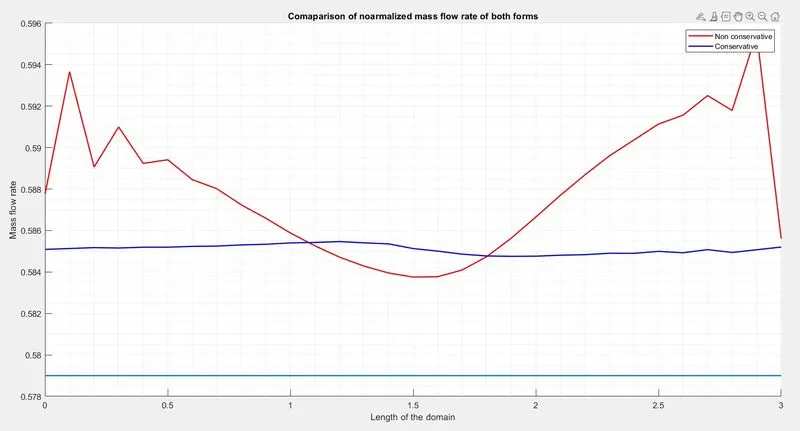
-From the above plot we saw that the non conservative form oscillate much but in conservative form output almost stable ,by this we can conclude that conservative attains stability is lesser number of iteration with earliest time.

GRID DEPENDENCE TEST-

-Comparision of solution after 1400 steps

Types of Form Grid no.(n) Density Pressure Temperature Mach number

Non conservative 31 0.638 0.534 0.836 0.9

61 0.637 0.532 0.835 0.9

Conservative 31 0.652 0.548 0.841 0.997

61 0.638 0.533 0.835 0.997

Analytic solution 0.634 0.833 0.528 1 (exact solution)

-Grid dependency is required to determine weather the program ca be solved faster,From the above table that the values are almost same in all premitive variable for both the form.

CONCLUSION-

From all the avove result we conclude that the conservative plot are closer to exat anaylatic plot and the conservative provide more accuracy for mass flow rate , but the non conservative form provides more accuracy for primitive variable .

Non conservation form has stable , accurate solution along the stimulation.