Project 2 - Rankine cycle Simulator

PROJECT :-

• To creat a Rankine cycle simulator using Matlab.
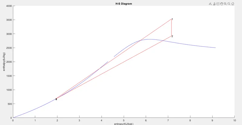
• To plot the T-s and H-s Curve

THEORY :-

• The Rankine cycle is an idealized thermodynamic cycle describing the process by which certain heat

engines such as steam turbine or reciprocating steam engines, allow mechanical work to be extracted

from a fluid as it moves between a heat source and heat sink.

• There are four proceses in the Rankine cycle ,as follow as

1. Process 1–2:- The working fluid is pumped from low to high pressure. As the fluid is a liquid at this stage,the pump requires little input energy. Process 1-2 is isentropic compression
2. Process 2–3: The high-pressure liquid enters a boiler, where it is heated at constant pressure by an external heat source to become a dry saturated vapour.It is constant pressure heat addition in boiler.
3. Process 3–4: The dry saturated vapour expands through a turbine generating power. This decreases temperature and pressure of the vapour, and some condensation may occur.It is isentropic expansion.
4. Process 4–1: The wet vapour then enters a condenser where it is condensed at a constant pressure become a saturated liquid. This is constant pressure heat rejection in condenser.

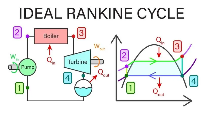
Figure-1(Ideal Rankine Cycle)

GOVERNING EQUATION :-

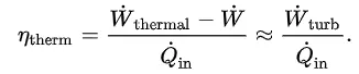
• The efficiency of simple rankine cyckle is defind as folloew as,

MAIN CODE :-

clear all 
close all
clc

disp('Ranking cycle simulator');
disp('1-2 = Iseentropic expansion in the turbine');
disp('2-3 = constant presure heat rejection by the condensor ');
disp('3-4 = isentropic compression of the pump');
disp('4-1 = Condtant presure heat addition by boiler ');

%inputs
t1 = input('Enter the Temprature at the turbine inlet(in degree celsius):');

p1 = input('Enter the presure at the turbine inlet(in bar):');
p2 = input('Enter the presure at the condenser (in bar):');

fprintf('rRESULTSrn');

%STAGE 1 (for iseentropic expansion in the turbine)
s1 = x_steam('s_pT',p1,t1);
h1 = x_steam('h_pT',p1,t1);

%stage 2 (for constant presure heat rejection by the condensor)
sf2 = x_steam('sL_p',p2);
sg2 = x_steam('sV_p',p2);
hf2 = x_steam('hL_p',p2);
hg2 = x_steam('hV_p',p2);

s2 = s1;
t2 = x_steam('Tsat_p',p2);

%Splitting the formula
x2 = ((s2-sf2)/(sg2-sf2));
h2 = hf2+(x2*(hg2-hf2));

%sage3 (isentropic compression of the pump)
p3 = p2;
t3 = x_steam('Tsat_p',p2);
s3 = x_steam('sL_p',p3);
h3 = x_steam('hL_p',p3);

%getting cp and cv value from x_steam
cp4 = x_steam('cpL_p',p3);
cv4 = x_steam('cvL_p',p3);
gamma = (cp4/cv4);
g = (gamma-1/gamma);

%Stage 4 (Condtant presure heat addition by boiler)
p4 = p1;
s4 = s3;
h4 = x_steam('h_ps',p4,s4);
t4 = t3*((p4/p3)^g);

%Turbine work
wt = h1-h2;
%Pump work
wp = h4-h3;
%Network
w_net = wt-wp;

%Heat in and out of the system
q_in = h1-h4;
q_out = h2-h3;

q_in = h1-h4;
q_out = h2-h3;

n = w_net/q_in;
np = n*100;

ssc = 3600/w_net;
tf_sat = x_steam('Tsat_p',p1);
sf_sat = x_steam('sL_p',p1);
hf_sat = x_steam('hL_p',p1);
sg_sat = x_steam('sV_p',p1);
hg_sat = x_steam('hV_p',p1);

%Plot figure 1
figure(1)
hold on 
temp = linspace(0,400,1000);
for i = 1:length(temp)
    AA(i) =x_steam('sL_T',temp(i));
end

for j =1:length(temp)
    BB(j)=x_steam('sV_T',temp(j));
end

plot(AA,temp,'color','b')
plot(BB,temp,'color','b')

temp = (x_steam('Tsat_p',p1));
t0 = linspace(temp,t1,300);
for i =  1:length(t0)
    c11(i)=x_steam('s_pt',p1,t0(i));
end
t5 = x_steam('Tsat_p',p4);
s5 = x_steam('sL_T',t5);

plot([s1 s2],[t1 t2],'color','r')
plot([s2 s3],[t2 t3],'color','r')
plot([s3 s4],[t3 t4],'color','r')
plot([s4 s5],[t4 t5],'color','r')
plot([sf_sat sg_sat],[tf_sat tf_sat],'color','b')
plot(c11,t0,'color','r')

title('T-S Diagram')
xlabel('entropy(KJ/kgk)')
ylabel('Temptature(k)')

text(s1,t1,'1');
text(s2,t2,'2');
text(s3,t3,'3');
text(s4,t4,'4');
text(s1,t5,'5');
text(sg_sat,tf_sat,'1s');

%Plotting Figure (2)
figure (2)
hold on
temp1= linspace(0,400,1000);
for i = 1:length(temp1)
    CC(i) =x_steam('hL_T',temp1(i));
end

for j =1:length(temp1)
    DD(j)=x_steam('hV_T',temp1(j));
end

plot(AA,CC,'color','b')
plot(BB,DD,'color','b')


plot([s1 s2],[h1 h2],'color','r')
plot([s2 s3],[h2 h3],'color','r')
plot([s3 s4],[h3 h4],'color','r')
plot([s4 s1],[h4 h1],'color','r')

title('H-S Diagram')
xlabel('entropy(KJ/kgk)')
ylabel('enthalpy(kJ/kg)')

text(s1,h1,'1');
text(s2,h2,'2');
text(s3,h3,'3');
text(s4,h4,'4');

%Printing the output

fprintf('at state point 1:n')
fprintf('P1 is : %f Barn',p1)
fprintf('T1 is : %f deg celsius',p1)
fprintf('T1 is :%f KJ/Kgn',h1)
fprintf('S1 is : % f KJ/KgKrn',s1)

disp('at state point 2:')
fprintf('P2 is : %f Barn',p2)
fprintf('T2 is : %f deg celsius',p2)
fprintf('H2 is : %f KJ/Kgn',h2)
fprintf('S2 is : %f KJ/KgKn',s2)
fprintf('X is : %f rn',x2)

disp('at state point 3:')
fprintf('P3 is : %f Barn',p3)
fprintf('T3 is : %f deg celsius400n',p3)
fprintf('H3 is : %f KJ/Kgn',h3)
fprintf('S2 is : %f KJ/KgKbn',s3)

disp('at state point 4:')
fprintf('P4 is : %f Barn',p4)
fprintf('T4 is : %f deg celsius',p4)
fprintf('H4 is : %f KJ/Kgn',h4)
fprintf('S4 is : %f KJ/KgKbn',s4)

fprintf('Wt : %f KJ/Kgn',p3)
fprintf('Wp : %f KJ/Kgn',p3)
fprintf('Wnet : %f KJ/Kgn',wp)
fprintf('Ntherm : %f %%n',n*100)
fprintf('SSC : %f KJ/KWhbn',ssc)

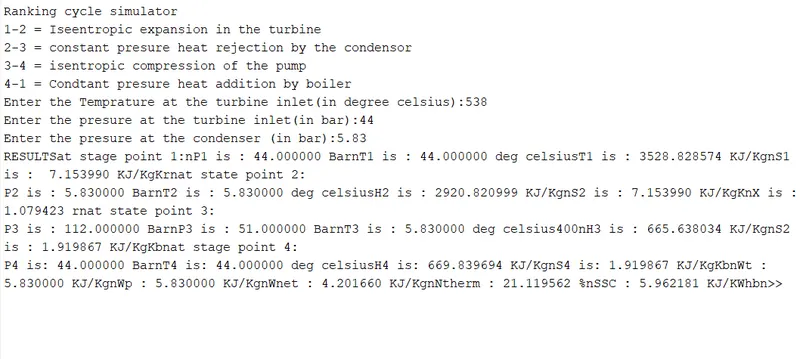
RESULTS:-

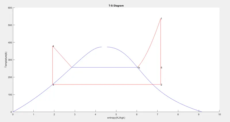
T-S Diagram:-

H-s Diagram:-

CONCLUSION:-

• The Rankine cycle plots have generated by calculating the state point efficiency and output pinted in command window.

OUTPUT IN COMMAND :-