Week 4.1 - Genetic Algorithm

PROJECT:-

• To optimise the stalagmite function and find the global maxima of the function

using matlab.

• Plot graphs for all studies and for F maximun and no of iteration.

THEORY:-

• The genetic algorithm is a method for solving both constrained and unconstrained optimization

that is based on natural selection, the process that drives biological evolution. The genetic algorithm

repeatedly modifies a population of individual solutions. At each step, the genetic algorithm selects

individuals at random from the current population to be parents and uses them to produce the for

the next generation. Over successive generations, the population "evolves" toward an optimal solution.

• You can apply the genetic algorithm to solve a variety of optimization problems that are not well suited

standard optimization algorithms, including problems in which the objective function is discontinuous,

nondifferentiable, stochastic, or highly nonlinear. The genetic algorithm can address problems of mixed

integer programming, where some components are restricted to be integer-valued.

• There are five phases in 'Ga' as follow,
• Initial population :- In this process the code gnerates random population and it is evaluate the fitness

of the member of the population according to which it forms new population based on number of

iteration performed.

• Fitness function :- It is the function define how the number of generation which are being formed

by the code with the fitness value of each member. Later these fitness value used for reproduction of

children.

• Selection :- In this phase we select the fitest individual, highest indivisual are more likely to select.

REPRODUCTION :-

There are two type of 'Ga' happens,

1. Crossover :- It is the process to generates off spring by meating a pair parents.
2. Mutation :- In a few off spring some of the genes can be subjected to mutation with low random

probability.

STALAGMITE FUNCTION :-

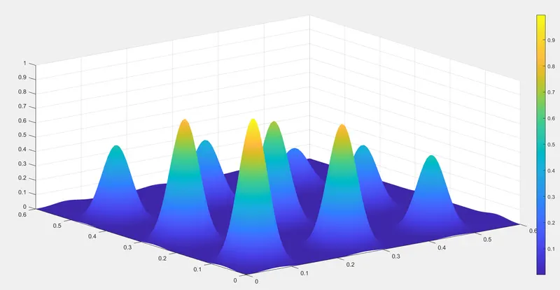
• A stalagmite function generally refers to the function with which we are generting values over thee stalagmite kind of surface for finding out the lacal maxima of the given function as follow,

`f(x,y)=f1x*f2x*f1y*f2y`

`f1x = (sin(5.1pix+0.5))^6`

`f1y= (sin(5.1piy+0.5))^6`

`f2x = exp[-4ln(2)*(x-0.667)^2/(0.64)]`

`f2y = exp[-4ln(2)*(y-0.667)^2/(0.64)]`

• Using this stalagmite function we are plotting the graph.

FUNCTION CODE:-

function [f] = stalagmite(input_vector)
x = input_vector(1);
y = input_vector(2);

f1x =(sin(5.1*pi*x + 0.5)).^6;
f1y =(sin(5.1*pi*y + 0.5)).^6;

f2x = exp(-4.*log(2)*((x-0.0667).^2/(0.64)));
f2y = exp(-4.*log(2)*((y-0.0667).^2/(0.64)));

f = -(f1x.*f2x.*f1y.*f2y);
end

MAIN CODE :-

clear all
close all
clc

%inputs for the search space of the function
x = linspace(0,0.6,150);
y = linspace(0,0.6,150);
[X,Y]=meshgrid(x,y);

% Number of itreation
num_case = 50;

%calling the stalagmite fuction
for i=1:length(x)
    for j=1:length(Y)
        input_vector(1)=X(i,j);
        input_vector(2)=Y(i,j);
        f(i,j)=stalagmite(input_vector);
    end
end
surf(x,y,-f);
shading interp

EXPLANATION OF MAIN CODE:-

• First we put some inputs for the search space of the function using linspace comand.
• Then we use the mesh comand and define the number of iteration
• Num_case is use to iterate the value of the optimum value of the function.
• Then we call the Stalagmite function which we have done previously.
• After that we use surf and shading comand to generate surface and remove the line produce by the mesh grid.

RESULTS:-

STUDY OF FIRST BEHAVIOUR WITHOUT BOUNDATION:-

%Static behaviour
%Calculating the study time using tic and toc comand
tic
for i=1:num_case

    [inputs,fopt(i)]=ga(@stalagmite,2);
    xopt(i)=inputs(1);
    yopt(i)=inputs(2);
end
study_time1=toc
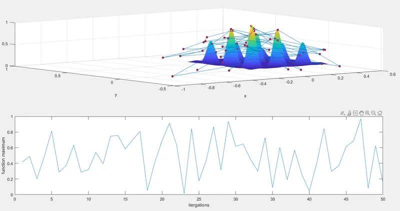
%Ploting unbounded inputs
figure(1)
subplot(2,1,1)

surf(x,y,-f)
hold on
shading interp
plot3(xopt,yopt,-fopt,'Marker','o','MarkerSize',5,'MarkerFaceColor','r');
xlabel('x')
ylabel('y')
grid on
subplot(2,1,2)
plot(-fopt);
xlabel('itergations')
ylabel('function maximum')

Using this program the results are not accurate as shown in below fig.

STUDY OF SECOND BEHAVIOUR WITH BOUNDATION:-

%Statistical behaviour(bounded)

tic
for j=1:num_case
    [inputs,fopt(j)]=ga(@stalagmite,2,[],[],[],[],[0;0],[1;1]);
    xopt(j)=inputs(1);
    yopt(j)=inputs(2);
end
study_time2=toc

%ploting
figure(2)

subplot(2,1,1)
hold on 
surf(x,y,-f)
shading interp
plot3(xopt,yopt,-fopt,'Marker','o','MarkerSize',5,'MarkerFaceColor','r')
xlabel('x')
ylabel('y')
grid on 
subplot(2,1,2)
plot(-fopt)
xlabel('iterations')
ylabel('function maximum')


   

RESULTS:-

STATISTICAL STUDY WITH INCREASE IN SIZE OF POPULATION:-

options=optimoptions('ga','PopulationSize',400);

tic
for k=1:num_case
    [inputs,fopt(k)]=ga(@stalagmite,2,[],[],[],[],[0;0],[1,;1],[],[],options);
    xopt(k)=inputs(1);
    yopt(k)=inputs(2);
end
study_time3=toc
%plotting
figure(3)

subplot(2,1,1)
hold on 
surf(x,y,-f)
shading interp
plot3(xopt,yopt,-fopt,'Marker','o','MarkerSize',5,'MarkerFaceColor','r')
xlabel('x')
ylabel('y')
grid on 
subplot(2,1,2)
plot(-fopt)
xlabel('iterations')
ylabel('function maximum')

EXPLANATION OF THE CODE:-

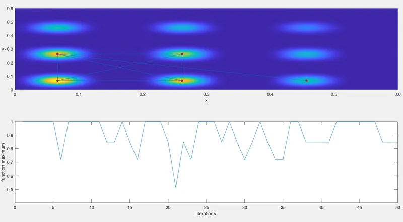
• In this program we are using optimoption command to increses the size of the population.
• This will help working on large set ,which will find the best fitness.

RESULTS:-

CONCLUSION:-

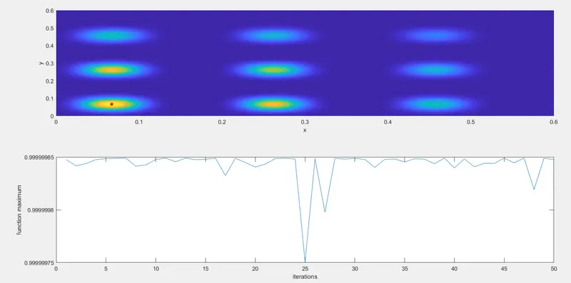
• Using this program we are able to plot 3 graphs as shown in figures and know ga is useful for optimizing the function.