Week 3 - Solving second order ODEs

PROJECT:-

--Solving second order differntial equation for calculating displacement and velocity

with respect to time using matlab.

-- Creat an animation of simple pendulum .

THEORY:-

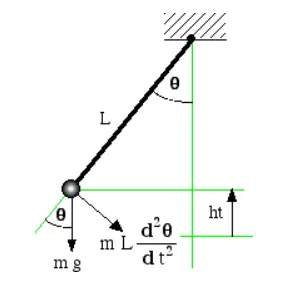
fig(1)

--Here is the the second order differntial equation

`(d^2theta)/dt^2+b/m*(d theta )/dt+g/l*sin theta`

transform the second order problem into two first order problems.

--first ode equatiion

`(d theta)/dt = theta2`

--second ode equation

`(d theta^2)/dt = -b/m*theta2-g/l*sin theta1`

-- EXPLANION OF THE CODE:-

-To solve the ode we have to take parameters as follow as,

Damping cooeficient(b)=0.05,Length(l) = 1,Mass(m) = 1,gravity(g )= 9.81

- Initial condition

angular displacement = 0, angular velocity= 3,time =0

-- Solving ode:-

To use ode45 solver we are creating a function a ode_function.

- providing the time limits and initial condition to ode45 syntax.

- Then we are using "for loop" , as the bob moves with a velocity and displacemet with

the given time period.

- At last we use movie command ti generate the anaimatio video.

MAIN CODE:-

close all
clear all
clc
 
% Inputs
%damping coefficient
b = 0.05;
%gravity
g = 9.81;
% lenght of the pendulum
l = 1;
% mass of the ball
m = 1;

% Initial condition 
% angular displacement and velocity
theta_0 = [0;3];

% Time point
t_span = linspace(0,20,200);

% Ode solver to solve second order ode
[t,results] = ode45(@(t,theta)ode_function(t,theta,b,g,l,m),t_span,theta_0);

plot(t,results(:,1))
hold on
plot(t,results(:,2))
grid on
title('damped harmonic motion of pendulum')
xlabel('time(sec)')
ylabel('angular velocity/displacement')

% Animating the motion of the pendulum
figure(2)

%counter comand
ct = 1;

for i = 1:length(results(:,1));
    
    %fixed coordinates of pendullum
    x0 = 0;
    y0 = 0;
    %moving coordinates of pendulum
    x1 = l*sin(results(i,1));
    y1 = -l*cos(results(i,1));
    % ploting
    plot([-3 3],[0 0],'LineWidth',2)
    hold on 
    plot([x0 x1],[y0 y1],'-o','MarkerSize',3,'LineWidth',2,'Color','r')
    axis([-1.5 1.5 -1.5 1.5])
    plot(x1,y1,'-o','MarkerSize',20,'MarkerFaceColor','b')
    pause(0.01)
    M(ct)=getframe(gcf)
    hold off
    ct = ct+1
end
% animation video
movie(M)
videofile= VideoWriter('simple_pendulum.avi','Uncompressed AVI')
open(videofile)
writeVideo(videofile,M)
close(videofile)

FUNCTION CODE:-

%function code for ode
function[dtheta_dt] = ode_function(t,theta,b,g,m,l)
theta1 = theta(1)
theta2 = theta(2)
dtheta1_dt =theta2;
dtheta2_dt = -(b/m)*theta2-(g/l)*sin(theta1);
dtheta_dt = [dtheta1_dt;dtheta2_dt];
end

OUTPUT:-

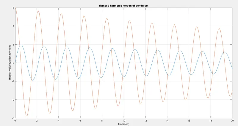
Youtube link for animatio video:-

https://youtu.be/oQF1ZuV61Jo

CONCLUSION:-

--Using the 2nd order differential equation we are now able to plot the damed harmonic motion

of pendulum and creat the animation video

error screnshot is below