Week 7 - Simulation of a 1D Super-sonic nozzle flow simulation using Macormack Method

OBJECTIVE: To simulate the isentropic flow through a quasi 1D subsonic-supersonic nozzle by both the conservation and non-conservation forms of the governing equations and sovle them using the MacCormack's technique.

THEORY: The governing equations of continuity,momentum and energy in terms of non-dimensional variables for quasi1D are expressed as,

Non-conservative Conitnuity equation:

`(delrho')/(delt') = -rho'((delV')/(delx')) -rho'V'((dellnA')/(delx'))-V'((delrho')/(delx'))`

Non-conservative Momentum equation:

`(delV')/(delt') = -V'((delV')/(delx'))-(1/gamma)((delT')/(delx')+((T')/(rho'))((delrho')/(delx')))`

Non-Conservative Energy equations:

`(delT')/(delx') = -V'((delT')/(delx'))-(gamma-1)T'[(delV')/(delx')+V'(del(lnA'))/(delx')]`

Conservative Continuity equation:

`(del(rho'A'))/(delt')+(del(rho'A'V'))/(delt') = 0`

Conservative Momentum equation:

`(del(rho'A'V'))/(delt')+(del[rho'A'(V')^2+(1/gamma)(rho'A')])/(delx') = (1/gamma)rho'((delA')/(delx'))`

Conservative Energy equation:

`(del[rho'((e')/(gamma-1) +(gamma/2)(V')^2)A'])/(delt')+(del[rho'((e')/(gamma-1) +(gamma/2)(V')^2)V'A'+rho'A'V'])/(delx') = 0`

We have taken the constant gamma value as 1.4

The MacCormack method is a widely used discretization scheme for the numerical solution of hyperbolic partial differential equations.

It is 2 phase method

In 1st phase we use the initial conditions to calculate the value for the predictive step. once we have predective step we do solution update, where with predicted derivative value of quantity updated values are calculated i.e. (quantity)* = (quantity)initial + deldeltp(quantity)*dt

using this value we calculate corrector step which is the 2nd phase after this we compute the avg of corrector and predictor step and use it to calculate the final values.

MATLAB CODES:

NON-CONSERVATIVE FUNCTION

function [mfr_nc,mfr_throat_nc] = non_conservative(L,n,nt,cfl)

x= linspace(0,L,n);
dx = x(2)-x(1);

%INITIAL CONDITIONS
rho = 1-0.3146*x;
T = 1-0.2314*x;
v=(0.1+1.09*x).*T.^0.5;
a=1+2.2*(x-1.5).^2;
M=v./(T.^0.5);
mfr=rho.*a.*v;
p=rho.*T;
g=1.4;

for z=1:31
    u=(T(z))^(1/2);
    dt(z)=cfl*dx/(u+v(z));
end
dt=min(dt);
for i=1:length(nt)
    rho_old=rho;
    T_old=T;
    v_old=v;
    for j=2:n-1
        %PREDICTOR STEP
        drho_dx = (rho(j+1)-rho(j))/dx;
        dv_dx = (v(j+1)-v(j))/dx;
        dT_dx = (T(j+1)-T(j))/dx;
        da_dx = (log(a(j+1))-log(a(j)))/dx;
        drho_dt_p(j)= -rho(j)*dv_dx-rho(j)*v(j)*da_dx-v(j)*drho_dx;
        dv_dt_p(j) = -v(j)*dv_dx - (1/g)*(dT_dx+(T(j)/rho(j))*drho_dx);
        dT_dt_p(j) = -v(j)*dT_dx - (g-1)*T(j)*(dv_dx+v(j)*da_dx);
        %UPDATING VALUES
        v(j) = v_old(j) + dv_dt_p(j)*dt;
        rho(j) = rho_old(j)+drho_dt_p(j)*dt;
        T(j) = T_old(j) + dT_dt_p(j)*dt;
        %CORRECTOR STEP
        drho_dx = (rho(j)-rho(j-1))/dx;
        dv_dx = (v(j)-v(j-1))/dx;
        dT_dx = (T(j)-T(j-1))/dx;
        da_dx = (log(a(j))-log(a(j-1)))/dx;
        drho_dt_c(j)= -rho(j)*dv_dx - rho(j)*v(j)*da_dx - v(j)*drho_dx;
        dv_dt_c(j) = -v(j)*dv_dx - (1/g)*(dT_dx+(T(j)/rho(j))*drho_dx);
        dT_dt_c(j) = -v(j)*dT_dx - (g-1)*T(j)*(dv_dx+v(j)*da_dx);
    end
    %AVERAGE PREDICTOR AND CORRECTOR
drho_dt_avg = 0.5*(drho_dt_p +drho_dt_c);
dv_dt_avg = 0.5*(dv_dt_p + dv_dt_c);
dT_dt_avg = 0.5*(dT_dt_p + dT_dt_c);
%FINAL VALUES
for k=2:n-1
    rho(k)=rho_old(k)+drho_dt_avg(k)*dt;
    v(k)=v_old(k)+dv_dt_avg(k)*dt;
    T(k)=T_old(k)+dT_dt_avg(k)*dt;
end
%BOUNDRY CONDITIONS
v(1)=2*v(2)-v(3);
v(n)=2*v(n-1)-v(n-2);
rho(n)=2*rho(n-1)-rho(n-2);
T(n)=2*T(n-1)-T(n-2);

p=rho.*T;
M=v./T.^0.5;
error(k) = abs(v(k)-v(k-1));
mfr = rho.*a.*v;
%VALUES AT THROAT i.e. AT MID OF NOZZLE
T_throat(i) = T(16);
rho_throat(i) = rho(16);
v_throat(i) = v(16);
M_throat(i)=M(16);
p_throat(i)=p(16);
error_throat(i)=error(16);
mfr_throat(i)=mfr(16);
if n==31
for ii = [1:50:201 700]
    if ii==i
        figure(1)
        plot(x,mfr)
        hold on
        title('NON-CONSERVATIVE FORM VARIATION OF MASS FLOW RATE INSIDE NOZZLE')
        xlabel('NOZZLE LENGTH')
        ylabel('MASS FLOW RATE')
    elseif i==1400
        plot(x,mfr)
        legend('1','51','101','201','700','1400')
    end
end
end
end
if n==31
    figure(2)
    plot(x,v,'b',x,p,'r',x,T,'k',x,rho,'m',x,M,'g',x,mfr,'c')
    ylim([-0.1 3.7])
    title(sprintf('TIME STEP = %d',i))
    xlabel('NOZZLE LENGTH')
    ylabel('NON DIMENSIONAL PARAMETERS')
    legend('Velocity','Pressure','Temperature','Density','Mach Number','Mass Flow Rate')
    title('NON-CONSERVATIVE FORM STEADY STATE DISTRIBUTION')
    
    figure(3)
    plot(nt,rho_throat)
    hold on
    plot(nt,v_throat)
    plot(nt,p_throat)
    plot(nt,T_throat)
    plot(nt,M_throat)
    plot(nt,mfr_throat)
    xlabel('TIMESTEPS(nt)')
    ylabel('NON DIMENSIONAL PARAMETERS')
    legend('Density','Velocity','Pressure','Temperature','Mach number','Mass flow rate')
    title('NON-CONSERVATIVE FORM TIME WISE VARIATION')
    
end
mfr_nc=mfr;
mfr_throat_nc=mfr_throat;
end

        
        
        

CONSERVATIVE FUNCTION

function [mfr_c,mfr_throat_c] = conservative(L,n,nt,cfl)
x=linspace(0,L,n);
dx=x(2)-x(1);
%INITIAL CONDITIONS
for ii=1:length(x)
    if(x(ii)<=0.5)
        rho(ii)=1;
        T(ii)=1;
    elseif (x(ii)>0.5) && (x(ii)<=1.5)
        rho(ii) = 1-0.366*(x(ii)-0.5);
        T(ii) = 1-0.167*(x(ii)-0.5)
    elseif (x(ii)>1.5) && (x(ii)<=3.5)
        rho(ii) = 0.634-0.3879*(x(ii)-1.5);
        T(ii)= 0.833-0.3507*(x(ii)-1.5);
    end
end
a=1+2.2*(x-1.5).^2;
g = 1.4;
%SOLUTION VECTORS
u1 = rho.*a;
u2 = 0.59*ones(1,n);
v=u2./u1;
u3 = u1.*((T./(g-1))+(g/2).*v.^2);

M = v./(T.^0.5);
mfr = rho.*a.*v;
p=rho.*T;

for z=1:31
    u=(T(z))^(1/2);
    dt(z) = cfl*dx/(u+v(z));
end
dt=min(dt);
for i=1:length(nt)
    u1_old=u1;
    u2_old=u2;
    u3_old=u3;
    for j = 2:n-1
        %FLUX
        f1=u2;
        f2=((u2.^2)./u1)+((g-1)/g)*(u3-((g/2)*(u2.^2)./u1));
        f3=((g.*u2.*u3)./u1)-((g*(g-1)/2)*(u2.^3)./(u1.^2));
        %SOURCE
        j1 = (1/g)*rho(j)*T(j)*((a(j+1)-a(j))/dx);
        %PREDICTOR
        du1_dt_p(j) = -(f1(j+1)-f1(j))/dx;
        du2_dt_p(j) = -(f2(j+1)-f2(j))/dx + j1;
        du3_dt_p(j) = -(f3(j+1)-f3(j))/dx;
        %UPDATING ITERATION VECTOR
        u1(j) = u1_old(j) +  du1_dt_p(j)*dt;
        u2(j) = u2_old(j) +  du2_dt_p(j)*dt;
        u3(j) = u3_old(j) +  du3_dt_p(j)*dt;
        
        rho=u1./a;
        T=(g-1).*(u3./u1-(g/2).*(u2./u1).^2);
        %UPDATING FLUX
        f1=u2;
        f2=((u2.^2)./u1)+((g-1)/g)*(u3-((g/2)*(u2.^2)./u1));
        f3=((g.*u2.*u3)./u1)-((g*(g-1)/2)*(u2.^3)./(u1.^2));
        
        %CORRECTOR 
        j2 = (1/g)*(rho(j)*(a(j)-a(j-1))/dx);
         du1_dt_c(j) = -(f1(j)-f1(j-1))/dx;
        du2_dt_c(j) = -(f2(j)-f2(j-1))/dx + j2;
        du3_dt_c(j) = -(f3(j)-f3(j-1))/dx;
    end
    %AVERAGE OF CORECTOR AND PREDICTOR
    du1_dt_avg = 0.5*(du1_dt_p +du1_dt_c);
du2_dt_avg = 0.5*(du2_dt_p + du2_dt_c);
du3_dt_avg = 0.5*(du3_dt_p + du3_dt_c);

for k = 2:n-1
    u1(k)=u1_old(k)+du1_dt_avg(k)*dt;
    u2(k)=u2_old(k)+du2_dt_avg(k)*dt;
    u3(k)=u3_old(k)+du3_dt_avg(k)*dt;
end
%BOUNDARY CONDITIONS
u1(1)=a(1);
u2(1)=2*u2(2)-u2(3);
u3(1)= u1(1)*(T(1)/(g-1)+(g*(u2(1)/u1(1))^2)/2);
u1(n)=2*u1(n-1)-u1(n-2);
u2(n)=2*u2(n-1)-u2(n-2);
u3(n)=2*u3(n-1)-u3(n-2);

%FINAL VALUES
rho=u1./a;
v=u2./u1;
T=(g-1).*(u3./u1-(g/2).*(u2./u1).^2);
p=rho.*T;
M=v./T.^0.5;
error(k) =abs(v(k)-v(k-1));
mfr=u2;

%VALUES AT THROAT i.e. AT MID OF NOZZLE
T_throat(i) = T(16);
rho_throat(i) = rho(16);
v_throat(i) = v(16);
M_throat(i)=M(16);
p_throat(i)=p(16);
error_throat(i)=error(16);
mfr_throat(i)=mfr(16);

if n==31
for ii = [1:50:201 700]
    if ii==i
        figure(4)
        plot(x,mfr)
        hold on
        title('CONSERVATIVE FORM VARIATION OF MASS FLOW RATE INSIDE NOZZLE')
        xlabel('NOZZLE LENGTH')
        ylabel('MASS FLOW RATE')
    elseif i==1400
        plot(x,mfr)
        legend('1','51','101','201','700','1400')
    end
end
end
end
if n==31
    figure(5)
    plot(x,v,'b',x,p,'r',x,T,'k',x,rho,'m',x,M,'g',x,mfr,'c')
    ylim([-0.1 3.7])
    title(sprintf('TIME STEP = %d',i))
    xlabel('NOZZLE LENGTH')
    ylabel('NON DIMENSIONAL PARAMETERS')
    legend('Velocity','Pressure','Temperature','Density','Mach Number','Mass Flow Rate')
    title('CONSERVATIVE FORM STEADY STATE DISTRIBUTION')

    figure(6)
    plot(nt,rho_throat)
    hold on
    plot(nt,v_throat);
    plot(nt,p_throat);
    plot(nt,T_throat);
    plot(nt,M_throat);
    plot(nt,mfr_throat);
    xlabel('TIMESTEPS(nt)')
    ylabel('NON-DIMENSIONAL PARAMETERS')
    legend('Density','Velocity','Pressure','Temperature','Mach Number','Mass flowrate')
    title('CONSERVATIVE FORM TIME WISE VARIATION')
end
mfr_c=mfr;
mfr_throat_c=mfr_throat;
end




        
        

MAIN CODE:

close all
clear all
clc

L=3;
n= 31;
nt = 1:1400;
cfl = 0.5;

    x = linspace(0,L,n);
    [mfr_nc,mfr_throat_nc] = non_conservative(L,n,nt,cfl);
    [mfr_c,mfr_throat_c] = conservative(L,n,nt,cfl);
   
    figure(7)
    subplot(2,1,1)
    plot(nt,mfr_throat_c,'b',nt,mfr_throat_nc,'r')
    xlabel('TIMESTEPS(nt)')
    ylabel('MASS FLOW RATE')
    legend('CONSERVATIVE FORM','NON-CONSERVATIVE FORM')
    title('MASS FLOW RATE AT THROAT (CONSERVATIVE vs NON-CONSERVATIVE)')
    subplot(2,1,2)
    plot(x,mfr_c,'b',x,mfr_nc,'r')
    hold on
    xlabel('NOZZLE LENGTH')
    ylabel('MASS FLOW RATE')
    legend('CONSERVATIVE FORM','NON-CONSERVATIVE FORM')
    title('MASS FLOW RATE IN NOZZLE (NON-CONSERVATIVE vs CONSERVATIVE')
    
   

    
    
    

OUTPUT PLOTS:

NON-CONSERVATIVE

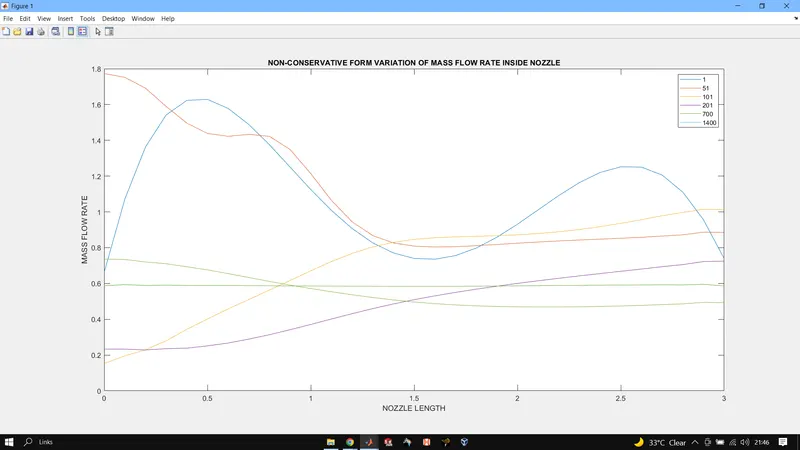
This shows the variation of ass flow rate throughout the nozzle at different time steps in our time marching process, it seems to average around 0.6.

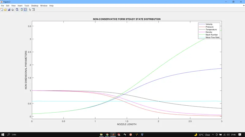
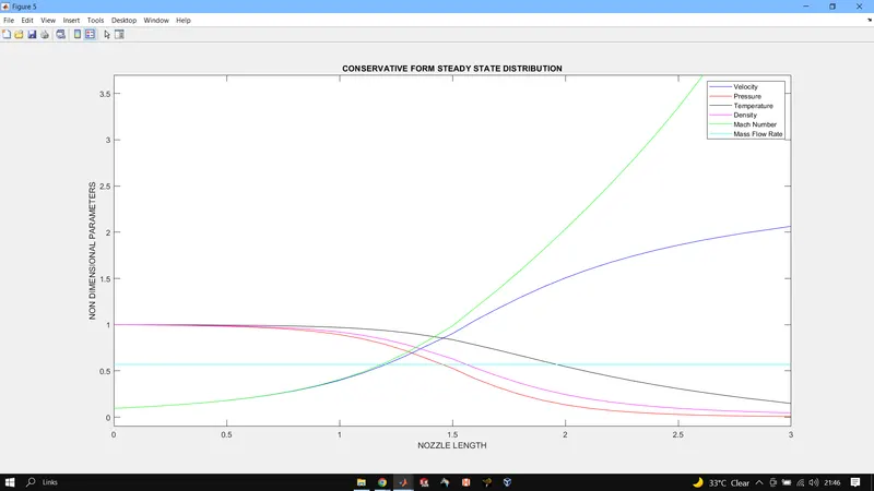
It shows steady state distribution of non-dimensional primitive variables at the end of time step.

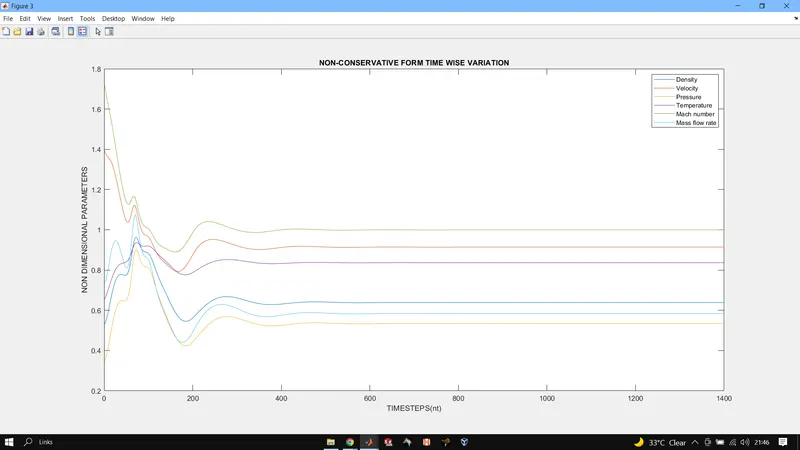
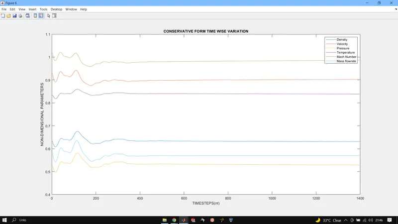
This shows time variation of primitive variables at throat, near to 400 time step we can see stable solutions.

CONSERVATIVE

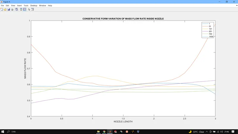
This shows the variation of ass flow rate throughout the nozzle at different time steps in our time marching process, it seems to average around 0.55.

This shows steady state distribution of primitive variables at the end of time step.

This shows time variation of primitive variables at throat, near to 400 time step we can see stable solutions.

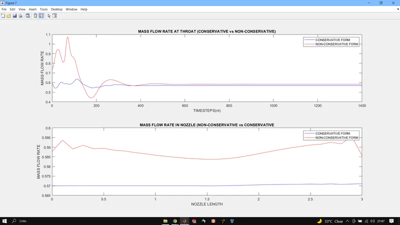
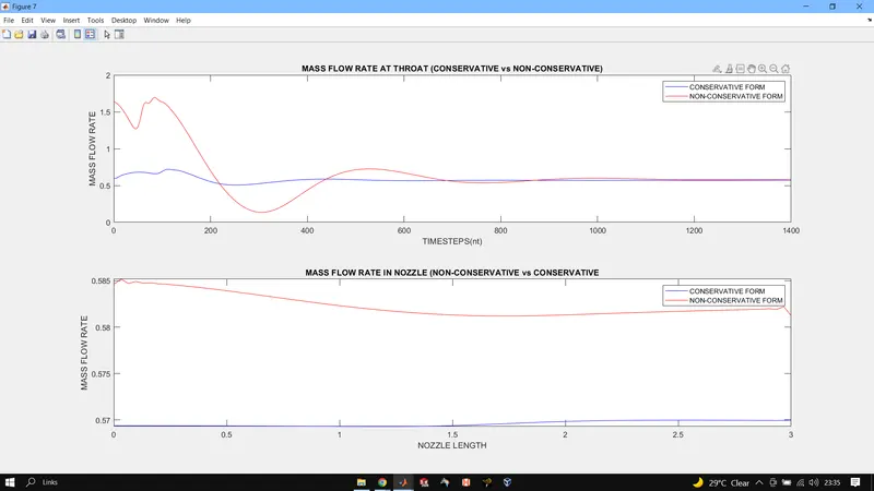
MASS FLOW RATE VARIATION

GRID INDEPENDENCE TEST

n = 31

n = 62

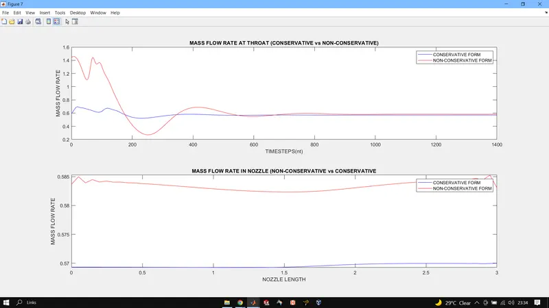
n = 93

We observe very small change in the value for solution for 3 different values of n(grid), the difference is of such a order that we can ignore it. Hence we can conlude that there isnt much vhange in the solution even when grid values are doubled or tripled hence our solutions arent much affected by the number of grids we have.

CONCLUSION: It can be said that at smaller time-steps behviour of non-conservative form shows a bit of unstable results but increase in time steps we see similar results of conservative and non-conservative approach.

Also we see difference in mass flow rate till 700 timesteps but after that the mass flow rate is constant and almost same for both, but before 700 we had fluctuations in non-conservative approach.

Though we didnt observe significant changes due to grid size but we can say that non-conservative form tends to become stable when grid size was increased tho the change was very small compared to change in grid size.