Week 7 - Simulation of a 1D Super-sonic nozzle flow simulation using Macormack Method
Intro
This study is looking at the implementation of the MacCormack method under two different setups to simulate a quasi-1D subsonic to supersonic nozzle flow scenario. This process will be commenced from first principles and into results.
Method
First-Principle Assumptions
The geometry is comprised of a nozzle of circular cross-section that varies across the length of the nozzle according to a parabolic function. This simple geometry allows us to make the following assumptions: The flow profile will show rotational symmetry, hence we only need to look at one dimension of axial flow to fully describe it. Then, we can also assume that this flow is invariable, hence removing the need to compute axial flow components. However, for the problem at hand to be described accurately, we still need to consider the cross-sectional area of the geometry, which only varies along its length. Hence, it is called a quasi-1D simulation, because we are using a term that cannot exist in one dimension.
Another important assumption that we are going to make is of the flow being inviscid. This is largely because we expect the inertial forces to be far larger than the viscous forces in the system, given that we are simulating supersonic airflow.
Moving forward, there are two main first-principle assumptions that we can make in this system of equations. These assumptions give us the last pieces of information that we need to derive the governing equations of the system, which describe conservation of mass, momentum and energy, and are to be implemented in our simulation.
One is by examining an infinitesimally small volume fixed in space and volume, through which fluid passes through with a certain pressure and velocity, and exerts stresses upon the surface of it. Starting from this setup, the conservative form of the governing equations is derived.
Meanwhile, we can also consider an infinitesimally small element of fixed mass moving with the flow with a certain velocity, and certain stresses are exerted upon its surface. This leads us to derive the non-conservative form of the governing equations. Both of these sets of assumptions are equally valid, however they lead to different setups later on.
Figure 1: Governing equations for a quasi-1D inviscid flow, shown in non-conservation (left) and conservation (right) form. The major difference between the two forms is that in the non-conservation form the primitive variables are simplified, whereas in the conservation form their components are fully expressed.
We will examine how both forms of the governing equations are implemented, and how their respective simulation setup unfolds.
On the algorithm used
The algorithm used to compute this is based on the MacCormack method. It employs two stages of first-degree approximations to reach a solution that exceeds the accuracy of such an approximation. At each time step, an intermediate solution is produced at the predictor step, which is then used to compute the corrector step terms and solution. The final solution is then found by averaging these two solutions.
This algorithm requires an initial set of primitive values that can undergo this iterative process. For each governing equation form, the initial conditions will be different. . In the non-conservative form, single linear functions are used to approximate each primitive variable. In the conservative form, single linear functions are used to approximate initial density and temperature within three separate segments of the geometry, and initial velocity is calculated based on initial density assuming initial mass flow rate is constant and uniform across the geometry. These initial conditions are expected to influence their respective simulations very differently.
The way this algorithm is applied also varies slightly across the two forms of governing equations. For the non-conservation form of the solution, this algorithm is applied directly onto the primitive variables to find their time-wise variation. However, for the conservation form if the equations, we substitute the primitive variables for a set of solution vectors and flux vectors onto which we apply the operations of the algorithm, composed of the primitive variables.
Based on the results obtained from the MacCormack method, consecutive time step snapshots of the primitive variables are plotted against distance along the nozzle, a sample of which is saved to disk and joined in video form.
Grid Independence Study
Before running our nozzle flow simulation, it is important that we make sure the process of geometry discretisation does not affect our results. This will be done by performing a grid independence study.
First, the simulation is run across grids of increasing node densities. The grid density is uniform across each grid iteration, starting off at 31 nodes and increasing by 30 nodes with every iteration (in order to retain the x values every 0.1 units and allow for book value comparisons).
Then, the difference between each of the primitive values across consecutive grids is computed, with the highest single value of which is recorded and plotted. Thus, the largest change in steady-state primitive values (in the plots it will be called “error”) is tracked. At the same time, primitive values at the throat region of the grid are recorded and plotted. The combination of these two plots will be used to observe the behaviour of the primitive values and whether or not they converge. An arbitrary accuracy will be employed to determine grid independence, and the grid selected will satisfy this accuracy criterion, whilst having the minimum number of grid points to do so.
In the interest of time, we will use the non-conservation form of the equations to check for grid independence, as they involve less operations and are therefore easier to obtain.
The code to perform the grid independence study is included below:
clear all;

close all;

clc;


error_rho=[];

error_v=[];

error_t=[];

q=100;


errorset_rho=zeros(1,31);

errorset_v  =zeros(1,31);

errorset_t  =zeros(1,31);


throat_rho=[];

throat_v=[];

throat_t=[];


allresults=zeros(q,31,3);


for n=31:30:(30*q +1)

    x = linspace(0,3,n);

    dx=x(2)-x(1);


    rho=1-0.3146*x;

    t = 1-0.2314*x; %Temperature!

    v = (0.1+1.09*x).*t.^0.5; % Velocity

    a=1+2.2*(x-1.5).^2;

    gamma=1.4;

    nt=500*(n-1)/30;

    dt=min((0.5).*dx./(sqrt(t)+v));

    titlelabels=["Pressure","Velocity","Temperature"];

    for k=1:nt


        errorset_rho_old=errorset_rho;

        errorset_v_old  =errorset_v;

        errorset_t_old  =errorset_t;


        rho_old=rho;

        v_old=v;

        t_old=t;


        for j=2:n-1  % Predictor Method


            %Forward difference spatial derivatives


            drhodx=(rho(j+1)-rho(j))/dx;

            dvdx=(v(j+1)-v(j))/dx;

            dtdx=(t(j+1)-t(j))/dx;

            dlogadx=(log(a(j+1))-log(a(j)))/dx;


            %Conservation equations


            drho_dt_p(j) = -rho(j)*dvdx -rho(j)*v(j)*dlogadx -v(j)*drhodx;

            dv_dt_p(j) = -v(j)*dvdx -(1/gamma) * (dtdx+t(j)*drhodx/rho(j));

            dt_dt_p(j) = -v(j)*dtdx-t(j)*(gamma-1)*(dvdx+v(j)*dlogadx);


            rho(j)=rho_old(j)+drho_dt_p(j)*dt;

            v(j)  =v_old(j)  +dv_dt_p(j)  *dt;

            t(j)  =t_old(j)  +dt_dt_p(j)  *dt;


        end


        for j=2:n-1  % Corrector Method


            %Backward difference spatial derivatives


            drhodx=(rho(j)-rho(j-1))/dx;

            dvdx=(v(j)-v(j-1))/dx;

            dtdx=(t(j)-t(j-1))/dx;

            dlogadx=(log(a(j))-log(a(j-1)))/dx;


            %Conservation equations


            drho_dt_c(j) = -rho(j)*dvdx -rho(j)*v(j)*dlogadx -v(j)*drhodx;

            dv_dt_c(j) = -v(j)*dvdx -(1/gamma) * (dtdx+t(j)*drhodx/rho(j));

            dt_dt_c(j) = -v(j)*dtdx-t(j)*(gamma-1)*(dvdx+v(j)*dlogadx);


        end


        drhodt=0.5*(drho_dt_c+drho_dt_p);

        dvdt=0.5*(dv_dt_p+dv_dt_c);

        dtdt=0.5*(dt_dt_c+dt_dt_p);


        for i=2:n-1

            rho(i)=rho_old(i)+drhodt(i)*dt;

            v(i)=v_old(i)+dvdt(i)*dt;

            t(i)=t_old(i)+dtdt(i)*dt;

        end


        v(1)=2*v(2)-v(3);


        v(n)=2*v(n-1)-v(n-2);

        t(n)=2*t(n-1)-t(n-2);

        rho(n)=2*rho(n-1)-rho(n-2);


    end

    for kk=1:31 %Taking primitive variable data at original 30 grid points (errorset data)

        errorset_rho(kk)=rho(1+(kk-1)*((n-1)/30));

        errorset_v(kk)  =  v(1+(kk-1)*((n-1)/30));

        errorset_t(kk)  =  t(1+(kk-1)*((n-1)/30));

    end


    %Calculating largest change in primitive variables and take it as error


    throat_rho = [throat_rho errorset_rho(16)];

      throat_v = [  throat_v errorset_v(16)  ];

      throat_t = [  throat_t errorset_t(16)  ];


    error_rho=[error_rho max(abs(errorset_rho(2:30)-errorset_rho_old(2:30)))];

    error_v  =[error_v   max(abs(  errorset_v(2:30)-  errorset_v_old(2:30)))];

    error_t  =[error_t   max(abs(  errorset_t(2:30)-  errorset_t_old(2:30)))];


    allresults((n-1)/30,:,1)=errorset_rho;

    allresults((n-1)/30,:,2)=errorset_v;

    allresults((n-1)/30,:,3)=errorset_t;


    n

end


figure(1);

xplot=30*linspace(1,100,100);

semilogy(xplot,error_rho,"r--",xplot,error_v,"g--",xplot,error_t,"b--")

grid on;

title("Number of Grid Points vs Final Time Step Error for Primitive Variables");

xlabel("Number of Grid Points");

ylabel("Error Magnitude");

labels=["Density","Velocity","Temperature"];

legend(labels);

probes=containers.Map({1,2,3},{throat_rho,throat_v,throat_t});


% Additional plot for closer data visualisation

figure(2);

for n=1:9:100

    for z=1:6

        subplot(3,2,z)

        if rem(z,2)==1

            plot(linspace(0,3,31),allresults(n,:,round(z/2)));

            hold on;

            grid on;

            xlabel("X-Distance");

            ylabel(labels(round(z/2)));

            title(sprintf("Steady-State %s across Grids of 30-3000 nodes",labels(round(z/2))));

            legend(["30 Grid Points","300 Grid Points","570 Grid Points","840 Grid Points","1110 Grid Points","1380 Grid Points","1650 Grid Points","1920 Grid Points","2190 Grid Points","2460 Grid Points","2730 Grid Points","3000 Grid Points"]);

        else

            if n==1

                plot(30*linspace(1,100,100),probes(round(z/2)));

                grid on;

                xlabel("Number of Grid Points");

                ylabel(sprintf("Throat %s",labels(round(z/2))));

            end

        end

    end

end
Upon running this code, the following figures are then obtained:
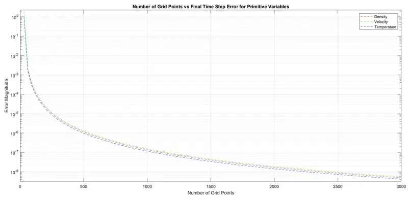
Figure 2: Rate of change of primitive variables (labelled error magnitude) against number of elements.
This shows that our choice of algorithm for the solution was good enough that the source of error is diminishing very quickly, so that it falls at a very high rate within few mesh iterations.
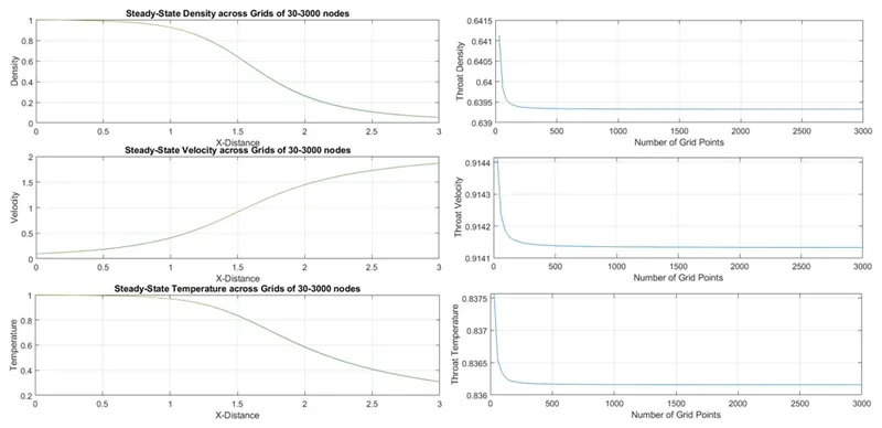
Figure 3: Steady-State primitive variable plots against distance and throat variable samples against number of grid points.
The Left-hand-side plots show that the solution has indeed converged smoothly and has taken the profile that is expected, and the right-hand side plots show the range of values obtained at the narrowest point in the throat - a particularly volatile sampling area. These ranges lie between 0.001 and 0.003 for all three variables, meaning that all results can provide least 2s.f. of accuracy.
However, to see how accurate our data is, we need to take a closer look at the plots.
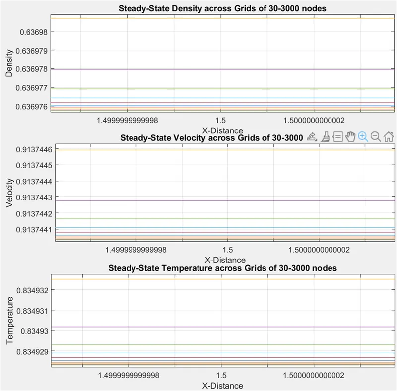
Figure 4: Zoom-in on the throat area node for the primitive variable plots. The top yellow line in each chart shows the 570 grid points plot for its respective variable.
This provides a better picture of how cumulative error decreases with increasing mesh size, showing an exponential decay trend. Here, we can see the range of values at the throat node is in the 1e-6 – 1e-7 order of magnitude, making all meshes whose data is depicted here accurate to at least 4s.f. and the densest meshes up to 6s.f. . This level of accuracy, however, is not necessary here. For the purpose of our study, 4s.f. is enough, therefore the 570 node mesh will be selected.
The simulations
Non-Conservative Form:
First, the non-conservative equations are discretised and used to solve for the primitive variables. Note: an abnormally large number of time steps was used to ensure that steady state is reached. This is performed by the code below:
clear all;

close all;

clc;


n=571;

x = linspace(0,3,n);

dx=x(2)-x(1);

rho=1-0.3146*x;

t = 1-0.2314*x; %Temperature!

v = (0.1+1.09*x).*t.^0.5; % Velocity

a=1+2.2*(x-1.5).^2;

gamma=1.4;

nt=1500*(n-1)/30;

dt=min((0.5).*dx./(sqrt(t)+v));

labels=["Density","Velocity","Temperature"];

mdot=zeros(nt,n);


for k=1:nt


    rho_old=rho;

    v_old=v;

    t_old=t;


    for j=2:n-1  % Predictor Method


        %Forward difference spatial derivatives


        drhodx=(rho(j+1)-rho(j))/dx;

        dvdx=(v(j+1)-v(j))/dx;

        dtdx=(t(j+1)-t(j))/dx;

        dlogadx=(log(a(j+1))-log(a(j)))/dx;


        %Conservation equations


        drho_dt_p(j) = -rho(j)*dvdx -rho(j)*v(j)*dlogadx -v(j)*drhodx;

        dv_dt_p(j) = -v(j)*dvdx -(1/gamma) * (dtdx+t(j)*drhodx/rho(j));

        dt_dt_p(j) = -v(j)*dtdx-t(j)*(gamma-1)*(dvdx+v(j)*dlogadx);


        rho(j)=rho_old(j)+drho_dt_p(j)*dt;

        v(j)  =v_old(j)  +dv_dt_p(j)  *dt;

        t(j)  =t_old(j)  +dt_dt_p(j)  *dt;


    end


    for j=2:n-1  % Corrector Method


        %Backward difference spatial derivatives


        drhodx=(rho(j)-rho(j-1))/dx;

        dvdx=(v(j)-v(j-1))/dx;

        dtdx=(t(j)-t(j-1))/dx;

        dlogadx=(log(a(j))-log(a(j-1)))/dx;


        %Conservation equations


        drho_dt_c(j) = -rho(j)*dvdx -rho(j)*v(j)*dlogadx -v(j)*drhodx;

        dv_dt_c(j) = -v(j)*dvdx -(1/gamma) * (dtdx+t(j)*drhodx/rho(j));

        dt_dt_c(j) = -v(j)*dtdx-t(j)*(gamma-1)*(dvdx+v(j)*dlogadx);


    end


    drhodt=0.5*(drho_dt_c+drho_dt_p);

    dvdt=0.5*(dv_dt_p+dv_dt_c);

    dtdt=0.5*(dt_dt_c+dt_dt_p);


    for i=2:n-1

        rho(i)=rho_old(i)+drhodt(i)*dt;

        v(i)=v_old(i)+dvdt(i)*dt;

        t(i)=t_old(i)+dtdt(i)*dt;

    end


    v(1)=2*v(2)-v(3);


    v(n)=2*v(n-1)-v(n-2);

    t(n)=2*t(n-1)-t(n-2);

    rho(n)=2*rho(n-1)-rho(n-2);


    data=[rho;v;t];


    figure(1)

    if rem(k,5) == 0

        for z=1:3

            subplot(3,1,z)

            plot(x,data(z,:));

            grid on;

            xlabel("X-Distance");

            ylabel(labels(z));

            title(sprintf("%s against Distance",labels(z)));

        end

        %saveas(gcf,sprintf("prim_vars_%04d",k/5),'png');

    end

    mdot(k,:)=rho.*v.*a;

end

save("dataset1.txt",mdot);
clear all;

close all;

clc;


n=571;

x = linspace(0,3,n);

dx=x(2)-x(1);


%Initialising primitive variables and terms used later on


for z=1:n

    if z > 286

        rho(z)=0.634-0.3879*(x(z)-1.5);

          t(z)=0.833-0.3507*(x(z)-1.5);

    else

        if z > 96

        rho(z)=1-0.366*(x(z)-0.5);

          t(z)=1-0.167*(x(z)-0.5);

        else

        rho(z)= 1;

          t(z)= 1;

        end

    end

end


a=1+2.2*(x-1.5).^2;

v = 0.59./(rho.*a);

gamma=1.4;

nt=1500*(n-1)/30;

A=figure;

df1dx=zeros(1,n-1);df2dx=zeros(1,n-1);df3dx=zeros(1,n-1);

du1dt_pred=zeros(1,n-1); du2dt_pred=zeros(1,n-1); du3dt_pred=zeros(1,n-1);

u1_pred=zeros(1,n-1); u2_pred=zeros(1,n-1); u3_pred=zeros(1,n-1);

f1_pred=zeros(1,n-1); f2_pred=zeros(1,n-1); f3_pred=zeros(1,n-1);

du1dt_corr=zeros(1,n-1); du2dt_corr=zeros(1,n-1); du3dt_corr=zeros(1,n-1);

u1_next=zeros(1,n); u2_next=zeros(1,n); u3_next=zeros(1,n);

mdot=zeros(nt,n);


%Initialising/updating solution and flux variables from primitive variables


u1=rho.*a;

u2=rho.*a.*v;

u3=rho.*( t/(gamma-1)+(gamma/2)*(v.*v) ).*a;

for z=1:nt


    dt=min((0.5).*dx./(sqrt(t)+v));


    f1=u2;

    f2=(u2.*u2)./u1 + ((gamma-1)/gamma)*(u3-(gamma/2)*(u2.*u2)./u1);

    f3=gamma*(u2.*u3)./u1 - gamma*(gamma-1)*0.5*(u2.*u2.*u2./u1./u1);


    for i=1:n-1 %Predictor Step

        df1dx(i)=(f1(i+1)-f1(i))/dx;

        df2dx(i)=(f2(i+1)-f2(i))/dx;

        df3dx(i)=(f3(i+1)-f3(i))/dx;

           j2(i)=1/gamma * rho(i) * t(i) * ((a(i+1)-a(i))/dx);


        du1dt_pred(i)=-df1dx(i);

        du2dt_pred(i)=-df2dx(i)+j2(i);

        du3dt_pred(i)=-df3dx(i);


        u1_pred(i)= u1(i) + du1dt_pred(i)*dt;

        u2_pred(i)= u2(i) + du2dt_pred(i)*dt;

        u3_pred(i)= u3(i) + du3dt_pred(i)*dt;

    end

    for i=1:n-1 %Updating flux vectors using predicted solution vectors

        f1_pred(i)=u2_pred(i);

        f2_pred(i)=(u2_pred(i)^2)./u1_pred(i) + ((gamma-1)/gamma)*(u3_pred(i)-(gamma/2)*(u2_pred(i)^2)/u1_pred(i));

        f3_pred(i)=gamma*(u2_pred(i)*u3_pred(i))/u1_pred(i) - gamma*(gamma-1)*0.5*(u2_pred(i)^3/u1_pred(i)^2);

    end

    for i=2:n-1 %Corrector Step

        df1dx(i)=(f1_pred(i)-f1_pred(i-1))/dx;

        df2dx(i)=(f2_pred(i)-f2_pred(i-1))/dx;

        df3dx(i)=(f3_pred(i)-f3_pred(i-1))/dx;

           j2(i)=1/gamma * rho(i) * t(i) * ((a(i)-a(i-1))/dx);


        du1dt_corr(i)=-df1dx(i);

        du2dt_corr(i)=-df2dx(i)+j2(i);

        du3dt_corr(i)=-df3dx(i);

    end


    %Final solution vectors at time step


    du1dt=0.5*(du1dt_pred+du1dt_corr);

    du2dt=0.5*(du2dt_pred+du2dt_corr);

    du3dt=0.5*(du3dt_pred+du3dt_corr);


    for i=2:n-1

        u1_next(i)=u1(i)+du1dt(i)*dt;

        u2_next(i)=u2(i)+du2dt(i)*dt;

        u3_next(i)=u3(i)+du3dt(i)*dt;

    end


    u1_next(1)=rho(1)*a(1);

    u2_next(1)=2*u2_next(2)-u2_next(3);

    u3_next(1)=u1(1)*( t(1)/(gamma-1) + (gamma/2)*(v(1)^2) );

    u1_next(n)=2*u1_next(n-1)-u1_next(n-2);

    u2_next(n)=2*u2_next(n-1)-u2_next(n-2);

    u3_next(n)=2*u3_next(n-1)-u3_next(n-2);


    %Updating primitive variables


    rho = u1_next./a;

      t = (gamma-1)*( (u3_next./u1_next) - (gamma/2)*(v.*v) );

      v = u2_next./u1_next;

      p = rho.*t;


    u1=u1_next;

    u2=u2_next;

    u3=u3_next;


    figure(A)


    subplot(3,1,1)

    plot(x,rho,"r-");

    title(sprintf("Primitive Variables along Nozzle length at Time = %.2f seconds",z*dt));

    grid on;

    ylabel("Density");

    subplot(3,1,2)

    plot(x,v,"g-");

    grid on;

    ylabel("Velocity");

    subplot(3,1,3)

    plot(x,t,"b-");

    grid on;

    xlabel("Distance Along Nozzle");

    ylabel("Temperature");

%     if rem(z,5)==0

%         saveas(gcf,sprintf("prim_vars_%04d",z/5),'png');

%     end

    mdot(z,:)=rho.*v.*a;


end
This yielded the animation below, showing the variation of primitive variables across time:
This time, the primitive variables reach their final form within less than 2000 time steps. No major discontinuities can be seen throughout the simulation, and visible steady state is reached within 5000 time steps. It is clear that initial conditions had a huge influence on the speed of convergence here, as they resembled the steady state much closer than the linear functions employed previously.
In both simulations, additional data on the mass flow rate along the nozzle was collected and exported manually (through the console) for use later on.
On the distribution of Mass flow rate
The primitive variable fields in both simulations were used to find the mass flow rate across space. To depict its variation in space and time, the following code was written:
clear all;
close all;
clc;

nc_data=load("dataset1.mat");
 c_data=load("dataset2.mat");
x=linspace(0,3,571);
dt=1.0717e-3;
a=figure;

 for z=1:10000
     figure(a)
     subplot(2,1,1)
     plot(x,nc_data.mdot(z,:))
     grid on;
     title(sprintf("Non-conservative dataset mass flow rate across nozzle, t= %.2f seconds",z*dt));
     ylabel("Mass Flow Rate");
     subplot(2,1,2)
     plot(x,c_data.mdot(z,:))
     grid on;
     title("Conservative dataset mass flow rate across nozzle");
     xlabel("X-Distance");
     ylabel("Mass Flow Rate");
     if rem(z,5)==0
        saveas(gcf,sprintf("mass_fig_%04d",z/5),'png');
     end
 end
This yielded the following results:
It can be seen here that the mass flow rate fluctuates in both simulations, these fluctuations being attenuated with time. There are some effects that are worth commenting on here.
First off, based on the difference in initial conditions, it is clear which lead to the most physically accurate results. The upper plot fluctuates between 2 and -0.05 (outflow through the inlet) across all points in space or time, showing the largest fluctuation of the two simulations. The lower plot shows far more stable behaviour, with mass flux only reaching between 0.45 and 1.2 . This is attributed to the initial conditions set, as the linear variations in primitive variables in the non-conservation form simulation are further from the steady state than the ones used in the other simulation.
The way mass flux varies with time resembles an attenuated wave moving in the direction of flow. This likely shows that the initial flow arrives in pulses before reaching a steady state. Such behaviour is further encouraged by absence of viscous forces, which would help to stabilise the flow rate.