Week 4.1 - Genetic Algorithm

There is a set of large multi-faceted problems that simple algorithms have a hard time solving. It is possible to solve these problems by taking an approach mimicking genetic processes, which encompass what we call a genetic algorithm (GA).

To solve a problem of a certain type of output, a population of solutions is first created. The individuals are assessed by a fitness function, upon the basis of which they undergo a series of processes representing natural selection processes. These processes are selection, reproduction, mutation, cross-over and migration, implemented through their own functions as part of the GA. Subsequent generations of solutions are thus driven toward certain values on the basis of the fitness function, ending upon certain criteria indicating solution convergence, such as the change in fitness function values falling below a certain tolerance level (1e-4 being the default).

In this study, the genetic algorithm, as implemented in MATLAB, will be used to find the maximum value in a plot resembling the shape of stalagmites. This determines the bounds of the domain as between 0 and 1 in every dimension. The maximum is found at [x,y]=[0.0671, 0.0671].

The code that does this is written below:

clear all;
close all;
clc;

% Creating the stalagmite function array; Note that this is given as
% negative, as the GA function finds function minima and we seek the maxima

x=linspace(0,1,150);
y=linspace(0,1,150);

[xx,yy]=meshgrid(x,y);
for i = 1:length(xx)
    for j = 1:length(yy)
        input(1) = xx(i,j);
        input(2) = yy(i,j);
        f(i,j) = stalagmite(input); % External stalagmite plot function
    end
end

% Computing stalagmite array minima using the genetic algorithm

% Setup 1: Unbound solution, 50 generations

n_cases = 50;
tic             % Recording computation time

for k = 1:n_cases
    [Inputs, Fopt(k)] = ga(@stalagmite,2); %Saving 
    xopt(k)=Inputs(1);
    yopt(k)=Inputs(2);
end

Fopt = -Fopt;   % Flipping the sign of the output for display purposes

Time_Study1 = toc % End of computation time

% Setup 2: Bounded Solution, 50 generations

tic
for k = 1:n_cases   
 [Inputs2, Fopt2(k)] = ga(@stalagmite,2,[],[],[],[],[0;0],[1;1]);
     xopt2(k) = Inputs2(1);
     yopt2(k) = Inputs2(2);
end

Fopt2 = -Fopt2;
Time_Study2 = toc

% Setup 3: Bounded solution, 50 generations, Population set to 200

options = optimoptions('ga', 'PopulationSize',200);
tic

for k = 1:n_cases
 [Inputs3, Fopt3(k)] = ga(@stalagmite,2,[],[],[],[],[0;0],[1;1],[],[],options);
     xopt3(k) = Inputs3(1);
     yopt3(k) = Inputs3(2);
end

Fopt3 = -Fopt3;
Time_Study3 = toc
f = -f;     % Restoring the sign of the stalagmite field

% Aggregating datasets

Fplots=containers.Map({1,2,3},{Fopt,Fopt2,Fopt3});
xplots=containers.Map({1,2,3},{xopt,xopt2,xopt3});
yplots=containers.Map({1,2,3},{yopt,yopt2,yopt3});
titles=["Unbounded Solution","Bounded Solution","Bounded Solution with Pop. 200"];

% Plotting results

figure;
for q=1:6
    subplot(3,2,q)
    hold on;
    if (rem(q,2) == 1)
        surfc(x,y,f);   % Original stalagmite function bird's eye view
        shading interp
        plot3(xplots(round(q/2)),yplots(round(q/2)),Fplots(round(q/2)),'bo','markersize',5,'markerfacecolor','r');
        % GA solutions overlay
        title(titles(round(q/2)));
    else
        plot(Fplots(round(q/2)),'b-','linewidth',1)  % Maximum value found in each generation
        xlabel('Iterations');
        ylabel('Function Maximum');
    end
end

rng('default');

The stalagmite plot created is the used as the function input for the genetic algorithm, as a 2-parameter function. From here, three arrangements are made:

• In the first arrangement, the algorithm is run without any additional inputs and alterations. This results in an initial field of solutions covering an area set by function defaults (the default is [-10;10] across each dimension)
• In the second arrangement, the algorithm is added boundaries, so that the initial population lies within the stalagmite function XY domain.
• In the third arrangement, additionally to the second arrangement, the algorithm is run with an initial population fixed at 200.

Each of these is then run for 250 instances. The total time it takes for these to run is also counted. The results are as follows (please note that the diagram extends to the right) :

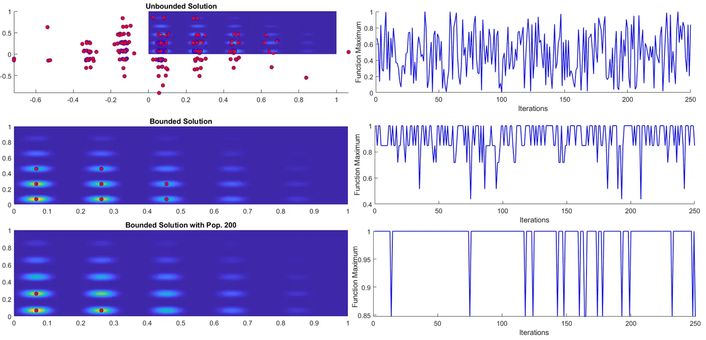
As it can be seen in the diagram above, the three GA arrangements show very different results. On average, each simulation took 0.0513s, 0.07591s and 0.2229s per solution. A 50% increase in computational time was incurred just by fixing the initial placement of the solutions. The additional alteration to the default initial population has further tripled the computation time.

Below is a depiction of the unbounded solutions zoomed in, with the maximum node in the stalagmite function highlighted:

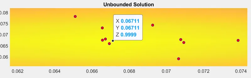
The unbound solution is the most inaccurate, with most solutions lying entirely outside the stalagmite domain. The range of solutions is roughly [-1,1] for both x and y coordinates, with solutions clustering around real or imaginary peaks of the stalagmite function plot. Only three solutions came within 3 s.f. (<0.9985) of the true solution, which is only 1.2% of the total number of solutions. This highlights the need for adding appropriate constraints to the GA - with all the GA options left as default and only the essential inputs, the chance of the GA finding the true solution are very slim.

Below is a depiction of the bounded solutions zoomed in onto the maximum found:

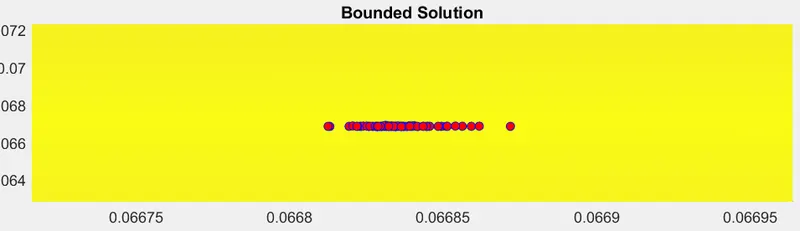
The second solution, however, was far more accurate, with all solutions converging onto the eight highest peaks. Amongst these, solutions at the highest peak show the exact Y value of the maximum, seeming to have converged on it completely. There is a narrow spread of values across the X axis, all of which are marked as having a height of 1. As there is no way for the solutions to improve, the convergence criterion of the fitness function is used to exit the GA. There is a range of values found because the maxima found here are the results of interpolation; a more finely distributed stalagmite function plot would likely depict these results better.

Below is a depiction of the bounded solutions of 200 total population zoomed in onto the maximum found:

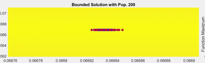
These were the most precise solutions between the three arrangements, with all but 16 solutions converging onto the peak, as depicted by the stalagmite function grid. As with the default settings bounded solution set, this set converged almost exactly onto the Y coordinate of the solution, however within a smaller x-coordinate range. These results show results about as accurate as the previous arrangement, however with diminishing returns in terms of precision, as they took nearly three times longer to compute. Still, these results are much more consistent, and likely do not require this many repetitions to provide a solution of high confidence level.