Week 3.5 - Deriving 4th order approximation of a 2nd order derivative using Taylor Table method

This study is looking at how Taylor series approximation precision is affected by the skew of data points used to compute them.

The following code took Taylor table coefficients to construct three fourth-order Taylor series approximation formulations of second order derivatives using centered, forward-skewed and backward-skewed data points. Then, these approximations were applied to the function `f(x)=e^x*cos(x)` using an array of finite difference values. The absolute error was then recorded.

clear all;
close all;
clc;

%Skewed-Right Solution Taylor Series coefficients:
M=[ 1,   1,  1,   1,    1;
    0,   1,  2,   3,    4;
    0, 0.5,  2, 4.5,    8;
    0, 1/6,4/3, 4.5, 64/6;
    0,1/24,2/3,27/8,64/6];
rhs=[0;0;1;0;0];
%Taylor Approximation coefficients: 
lhs=(M^-1)*rhs; 

%Skewed-Left Solution:
N=[1,   1,   1,   1,  1;
   0,  -1,  -2,  -3, -4;
   0, 0.5,  2 , 4.5,  8;
   0,-1/6,-4/3,-4.5,-64/6;
   0,1/24, 2/3,27/8, 64/6];

lhs2=(N^-1)*rhs;

%analytical function;
%f''(x)=fexercise(x)= -2*exp(x)*sin(x)

%Centered Solution:
lhs3=[-1;16;-30;16;-1]/12;%I solved this on paper, as matrix inversion doesn't work in this case.
x=pi/6;
dxset=linspace(pi/50,pi/4000,20);
analytical_derivative=-2*exp(x)*sin(x);

for i=1:20
    dx=dxset(i);
    bdarray = [fexercise(x)*lhs(1);fexercise(x-dx)*lhs(2);fexercise(x-2*dx)*lhs(3);fexercise(x-3*dx)*lhs(4);fexercise(x-4*dx)*lhs(5)]/(dx^2);
    fdarray = [fexercise(x)*lhs2(1);fexercise(x+dx)*lhs2(2);fexercise(x+2*dx)*lhs2(3);fexercise(x+3*dx)*lhs2(4);fexercise(x+4*dx)*lhs2(5)]/(dx^2);
    cdarray = [fexercise(x-2*dx)*lhs3(1);fexercise(x-dx)*lhs3(2); fexercise(x)*lhs3(3) ;fexercise(x+dx)*lhs3(4);fexercise(x+2*dx)*lhs3(5)]/(dx^2);
    backward_difference = sum(bdarray);
     forward_difference = sum(fdarray);
     central_difference = sum(cdarray);
    FDError  = abs(forward_difference  - analytical_derivative);
    BDError  = abs(backward_difference - analytical_derivative);
    CDError  = abs(central_difference  - analytical_derivative);
    bdset(i) = BDError;
    fdset(i) = FDError;
    cdset(i) = CDError;

    aaout=[bdset; fdset; cdset]
end

gradients = [sum(log(bdset))/sum(log(dxset));sum(log(fdset))/sum(log(dxset));sum(log(cdset))/sum(log(dxset))];

legendlabels=["Backward Difference Method","Forward Difference Method","Central Difference Method"]
figure;
plot(log10(dxset),log10(bdset),'rx',log10(dxset),log10(fdset),'bx',log10(dxset),log10(cdset),'gx')
xlabel("Finite Difference Order of Magnitude")
ylabel("Error Order of Magnitude")
grid on;
legend(legendlabels);

Finally, a loglog plot of the absolute error against the finite difference magnitude was used to extract the order of accuracy of our approximations based on the resulting gradient. As expected, the gradients were approximately equal to 4 and 3 for the centered and skewed data based formulas respectively. In each case, this indicates five data points were used for the approximation, hence fourth order approximations.

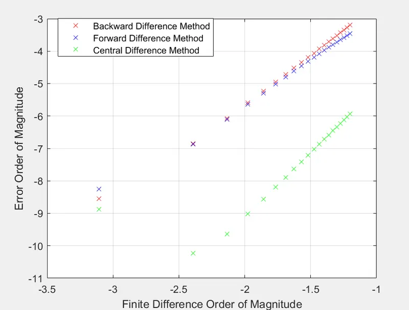
The approximations show predictable results, with the centered data scheme approximation showing the smallest error. However, an argument can be made in favour of using skewed data scheme formulas. It is often the case that these approximations are defined by the spatial domain and the configuration of nodes used to define it. At domain boundaries, the domain does not contain the nodes necessary to use a centered data scheme for numerical approximations. Thus, skewed Taylor approximations are necessary to obtain values in these areas.