Week 7 - Simulation of a 1D Super-sonic nozzle flow simulation using Macormack Method
Simulation of a 1D Super-sonic nozzle flow simulation using Macormack Method:
The Macormack method is a widely used discretization scheme for the numerical solution of hyperbolic partial differential equations.
The MacCormack method is a variation of the two-step Lax–Wendroff scheme but is much simpler in application. To illustrate the algorithm, consider the following first order hyperbolic equation
`(delu)/(delt)+a*(delu)/(delx)=0`
The application of MacCormack method to the above equation proceeds in two steps; a predictor step which is followed by a corrector step.
Predictor step:
In the predictor step, a "provisional" value of u at time level n+1 is estimated as follows
- `u_i^(n+1) = u_i^n-a(Deltat)/(Deltax)(u_(i+1)^n-u_i^n)`
The above equation is obtained by replacing the spatial and temporal derivatives in the previous first order hyperbolic equation using forward differences.
Corrector step:
In the corrector step, the predicted value `u_i^(n+1)` is corrected according to the equation
- ``u_i^(n+1) = u_i^(n+1/2)-a(Deltat)/(2Deltax)(u_(i)^(n+1)-u_(i-1)^(n+1`
Note that the corrector step uses backward finite difference approximations for spatial derivative. The time-step used in the corrector step is `(Deltat)/2` in contrast to the `Deltat` used in the predictor step.
Replacing the `u_i^(n+1/2)` term by the temporal average
- `u_i^(n+1/2) = (u_i^n+u_i^(n+1))/2`
to obtain the corrector step as
- `u_i^(n+1) = (u_i^n+u_i^(n+1))/2-a(Deltat)/(2Deltax)(u_(i)^(n+1)-u_(i-1)^(n+1))`
Main program:
The functions for the conservative and non conservative form are called and the comparison of mass flow rates between both forms is plotted.
clear all
close all
clc


%Inputs
n = 31;
x = linspace(0,3,n);
dx = x(2)-x(1);
gamma = 1.4;
throat = round(n/2);


%Analytical solution
a = 1+(2.2*(x-1.5).^2);
b = a*-1;
m = 0;

%Finding the mach number at eaxh points through out the nozzle
%Till the throat

for i = 1:throat
    residual = 1;
while residual > 1e-9
    m = m + 1e-4;
    residual = ((1/m^2)*((2/(gamma+1))*(1+((gamma-1)/2)*m^2))^((gamma+1)/(gamma-1)))-a(i)^2;
end
mach_number(i) = m;
end

%From throat to the exit
for i = (throat+1):n
    residual = 1;
while residual > 1e-9
    m = m + 1e-4;
    residual = ((1/m^2)*((2/(gamma+1))*(1+((gamma-1)/2)*m^2))^((gamma+1)/(gamma-1)))-a(i)^2;
    residual  = residual*-1;
end
mach_number(i) = m;
end


t  = (1+((gamma-1)/2).*mach_number.^2).^(-1);
rho = (1+((gamma-1)/2).*mach_number.^2).^(-1/(gamma-1))
p = rho.*t;


%Calling the functions
%Non conservation form
m_nc = Non_conservation_form(n,x,dx,gamma,throat)

%Conservation form
m_c = Conservation_form(n,x,dx,gamma,throat)

%Plotting Comparison of mass flow rates between the two forms
figure(9)
plot(x,m_nc)
hold on
plot(x,m_c)
xlabel('Nozzle length')
ylabel('Mass flow rate')
legend('Non conservation form','Conservation form')
title('Comparison of mass flow rates between the two forms')
Functions:
function m = Non_conservation_form(n,x,dx,gamma,throat)


%Calculate initial profiles
rho = 1-0.3146*x;%Density
t = 1-0.2314*x; %t = temperature
v = (0.1+1.09*x).*t.^0.5;%Velocity

%Area
a = 1+2.2*(x-1.5).^2;

%Time step
nt = 1400;
dt = 0.02;

%CFL number calculation
CFL = max((v+sqrt(t))*dt/dx);

%Outer time loop
for k = 1:nt

     %Copying old values
     rho_old = rho;
     v_old = v;
     t_old = t;

     %predictor method
     for j = 2:n-1

        dvdx = (v(j+1)-v(j))/dx;
        drhodx = (rho(j+1)-rho(j))/dx;
        dtdx = (t(j+1)-t(j))/dx;
        dlog_a_dx = (log(a(j+1))-log(a(j)))/dx;

         %Continuity equation
         drhodt_p(j) = -rho(j)*dvdx-rho(j)*v(j)*dlog_a_dx-v(j)*drhodx;

         %Momentun equation
         dvdt_p(j) = -v(j)*dvdx-(1/gamma)*(dtdx+(t(j)/rho(j))*drhodx);

         %Energy equation
         dtdt_p(j) = -v(j)*dtdx-(gamma-1)*(dvdx+v(j)*dlog_a_dx);

         %Solution update
         eho(j) = rho(j)+drhodt_p(j)*dt;
         t(j) = t(j)+dtdt_p(j)*dt;
         v(j) = v(j)+dvdt_p(j)*dt;
     end

      %Corrector method
      for j = 2:n-1

        dvdx = (v(j)-v(j-1))/dx;
        drhodx = (rho(j)-rho(j-1))/dx;
        dtdx = (t(j)-t(j-1))/dx;
        dlog_a_dx = (log(a(j))-log(a(j-1)))/dx;

         %Continuity equation
         drhodt_c(j) = -rho(j)*dvdx-rho(j)*v(j)*dlog_a_dx-v(j)*drhodx;

         %Momentun equation
         dvdt_c(j) = -v(j)*dvdx-(1/gamma)*(dtdx+(t(j)/rho(j))*drhodx);

         %Energy equation
         dtdt_c(j) = -v(j)*dtdx-(gamma-1)*(dvdx+v(j)*dlog_a_dx);


     end


     %compute the average time derivative
     dvdt = 0.5*(dvdt_p+dvdt_c);
     drhodt = 0.5*(drhodt_p+drhodt_c);
     dtdt = 0.5*(dtdt_p+dtdt_c);

     %Final solution update
     for i = 2:n-1
         rho(i) = rho_old(i)+drhodt(i)*dt;
         v(i) = v_old(i)+dvdt(i)*dt;
         t(i) = t_old(i)+dtdt(i)*dt;
     end
     %Apply boundary conditions
     %Inlet
     v(1) = 2*v(2)-v(3);

     %Outlet
     v(n) = 2*v(n-1)-v(n-2);
     rho(n) = 2*rho(n-1)-rho(n-2);
     t(n) = 2*t(n-1)-t(n-2);

     %Pressure
     p = rho.*t;

     %Mach number
     M = v./sqrt(t);

     %Mass flow rate
     m = rho.*a.*v;

    %Plotting Variation of mass flow rate at different time steps
     figure(4)
     hold on
     if k == 1
         plot(x,m);
     end
    if k == 1
         plot(x,m);
     end
    if k == 50
         plot(x,m);
     end
    if k == 250
         plot(x,m);
     end
    if k == 500
         plot(x,m);
     end
    if k == 750
         plot(x,m);
     end
    if k == 1400
         plot(x,m);
     end

    %Values at the throat
    rho_th(k) = rho(throat);
    v_th(k) = v(throat);
    t_th(k) = t(throat);
    p_th(k) = p(throat);
    M_th(k) = M(throat);

end
xlabel('Nozzle length')
ylabel('Mass flow rate')
legend('1dt','50dt','250dt','500dt','750dt','1400dt')
title('Variation of mass flow rate at different time steps (Non conservation form)')

%Plotting Steady state primitive variable profile
figure(1)
 subplot(5,1,1)
     plot(x,v)
     xlabel('Nozzle length')
     ylabel('velocity')
     title('Steady state primitive variables profile (Non conservation form)')

     subplot(5,1,2)
     plot(x,rho)
     xlabel('Nozzle length')
     ylabel('Density')


     subplot(5,1,3)
     plot(x,t)
     xlabel('Nozzle length')
     ylabel('Temperature')

     subplot(5,1,4)
     plot(x,p)
     xlabel('Nozzle length')
     ylabel('Pressure')

     subplot(5,1,5)
     plot(x,M)
     xlabel('Nozzle length')
     ylabel('Mach number')

     %Plotting Transient variation of primitive variables at throat
     figure(2)
     subplot(5,1,1)
     plot(v_th)
     xlabel('time step')
     ylabel('velocity')
     title('Transient variation primitive variables at throat (Non conservation form)')

     subplot(5,1,2)
     plot(rho_th)
     xlabel('time step')
     ylabel('Density')


     subplot(5,1,3)
     plot(t_th)
     xlabel('time step')
     ylabel('Temperature')

     subplot(5,1,4)
     plot(p_th)
     xlabel('time step')
     ylabel('Pressure')

     subplot(5,1,5)
     plot(M_th)
     xlabel('time step')
     ylabel('Mach number')

     %Plotting steady state mass flow rate
     figure(3)
     plot(x,m)
     xlabel('length')
     ylabel('Mass flow rate')
     title('Steady state mass flow rate (Non conservation form)')

end
function m = Conservation_form(n,x,dx,gamma,throat)
%Initial conditions
for i = 1:n
if x(i)>=0 && x(i) <= 0.5
rho(i)= 1;
t(i) = 1;
elseif x(i) > 0.5 && x(i) <= 1.5
rho(i) = 1 - 0.366*(x(i)-0.5);
t(i) = 1 - 0.167*(x(i)-0.5);
elseif x(i) > 1.5 && x(i) <= 3.5
rho(i) = 0.634 - 0.3879*(x(i)-1.5);
t(i) = 0.833 - 0.3507*(x(i)-1.5);
end
end
%Nozzle Area
a = 1 + 2.2*(x - 1.5).^2;
%Velocity
v = 0.59./(rho.*a);%(Assuming constant mass flow rate)
%Pressure
p = rho.*t;
%Solution vectors
U1 = rho.*a;
z = ones(1,n);
U2 = 0.59.*z;
U3 = U1.*(t/(gamma-1)+(gamma/2).*v.^2);
%Time step
nt = 1400;
%CFL number
CFL = 0.5;
%Outer time loop
for k = 1:nt
%Adaptive time step
dt = max((CFL.*dx)./(v+sqrt(t)))
%Copying old values of solution vectors
U1_old = U1;
U2_old = U2;
U3_old = U3;
%Initializing flux variables
F1 = U2;
F2 = ((U2.^2)./U1)+((gamma-1)/gamma)*(U3-(gamma/2)*((U2.^2./U1)));
F3 = gamma*U2.*U3./U1-0.5*gamma*(gamma-1)*(U2.^3./U1.^2);
%predictor method
for j = 2:n-1
%Continuity equation
dU1dt_p(j) = -(F1(j+1)-F1(j))/dx;
%Source term
J2(j) = (1/gamma)*rho(j)*t(j)*(a(j+1)-a(j))/dx;
%Momentun equation
dU2dt_p(j) = -(F2(j+1)-F2(j))/dx+J2(j);
%Energy equation
dU3dt_p(j) = -(F3(j+1)-F3(j))/dx;
%Solution update
U1(j) = U1(j)+dU1dt_p(j)*dt;
U2(j) = U2(j)+dU2dt_p(j)*dt;
U3(j) = U3(j)+dU3dt_p(j)*dt;
end
%Primitive variables
rho = U1./a;
t = (gamma-1)*(U3./U1-(gamma/2)*(U2./U1).^2);
%Reinitializing flux variables
F1 = U2;
F2 = ((U2.^2)./U1)+((gamma-1)/gamma)*(U3-(gamma/2)*((U2.^2./U1)));
F3 = gamma*U2.*U3./U1-0.5*gamma*(gamma-1)*(U2.^3./U1.^2);
%Corrector method
for j = 2:n-1
%Continuity equation
dU1dt_c(j) = -(F1(j)-F1(j-1))/dx;
%Source term
J2(j) = (1/gamma)*rho(j)*t(j)*(a(j)-a(j-1))/dx;
%Momentun equation
dU2dt_c(j) = -(F2(j)-F2(j-1))/dx+J2(j);
%Energy equation
dU3dt_c(j) = -(F3(j)-F3(j-1))/dx;
end
%compute the average time derivative
dU1dt = 0.5*(dU1dt_p+dU1dt_c);
dU2dt = 0.5*(dU2dt_p+dU2dt_c);
dU3dt = 0.5*(dU3dt_p+dU3dt_c);
%Final solution update
for i = 2:n-1
U1(i) = U1_old(i)+dU1dt(i)*dt;
U2(i) = U2_old(i)+dU2dt(i)*dt;
U3(i) = U3_old(i)+dU3dt(i)*dt;
end
%Apply boundary conditions
%Inlet
U1(1) = a(1);
U2(1) = 2*U2(2) - U2(3);
U3(1) = U1(1)*(t(1)/(gamma-1)+0.5*gamma*v(1)^2);
%Outlet
U1(n) = 2*U1(n-1)-U1(n-2);
U2(n) = 2*U2(n-1)-U2(n-2);
U3(n) = 2*U3(n-1)-U3(n-2);
%Final update of primitive variables
rho = U1./a;
v = U2./U1;
t = (gamma-1).*(U3./U1-(gamma/2).*(U2./U1).^2);
p = rho.*t;
M = v./t.*0.5;
m = U2;
%Primitive variables at the throat
rho_th(k) = rho(throat);
v_th(k) = v(throat);
t_th(k) = t(throat);
p_th(k) = p(throat);
M_th(k) = M(throat);
%Plotting Variation of mass flow rate at different time steps
figure(8)
hold on
if k == 1
plot(x,m);
end
if k == 50
plot(x,m);
end
if k == 250
plot(x,m);
end
if k == 500
plot(x,m);
end
if k == 750
plot(x,m);
end
if k == 1400
plot(x,m);
end
end
xlabel('Nozzle length')
ylabel('Mass flow rate')
legend('1dt','50dt','250dt','500dt','750dt','1400dt')
title('Variation of mass flow rate at different time steps (Conservation form)')
%Plotting Steady state primitive variable profile
figure(5)
subplot(5,1,1)
plot(x,v)
xlabel('Nozzle length')
ylabel('velocity')
title('Steady state primitive variables profile (Conservation form)')
subplot(5,1,2)
plot(x,rho)
xlabel('Nozzle length')
ylabel('Density')
subplot(5,1,3)
plot(x,t)
xlabel('Nozzle length')
ylabel('Temperature')
subplot(5,1,4)
plot(x,p)
xlabel('Nozzle length')
ylabel('Pressure')
subplot(5,1,5)
plot(x,M)
xlabel('Nozzle length')
ylabel('Mach number')
%Plotting Transient variation of primitive variables at throat
figure(6)
subplot(5,1,1)
plot(v_th)
xlabel('time step')
ylabel('velocity')
title('Transient variation of primitive variables at throat (Conservation form)')
subplot(5,1,2)
plot(rho_th)
xlabel('time step')
ylabel('Density')
subplot(5,1,3)
plot(t_th)
xlabel('time step')
ylabel('Temperature')
subplot(5,1,4)
plot(p_th)
xlabel('time step')
ylabel('Pressure')
subplot(5,1,5)
plot(M_th)
xlabel('time step')
ylabel('Mach number')
%Plotting steady state mass flow rate
figure(7)
plot(x,m)
xlabel('length')
ylabel('Mass flow rate')
title('Steady state mass flow rate (Conservation form)')
endPlots:
Non conservation form:
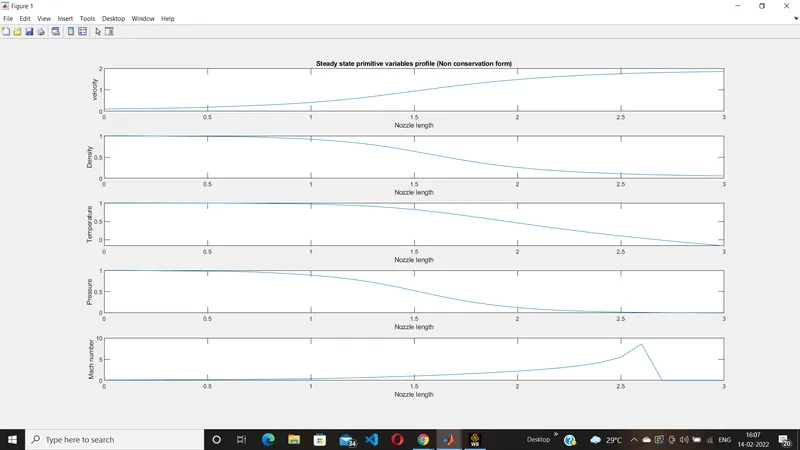
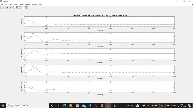
The above plots are drawn for each parameters such as Mach number,Density,Pressure,temperature for each time steps.
Initially, the values of all the parameters are very high and there are instabilities.And as the time step increases the plots become stable.
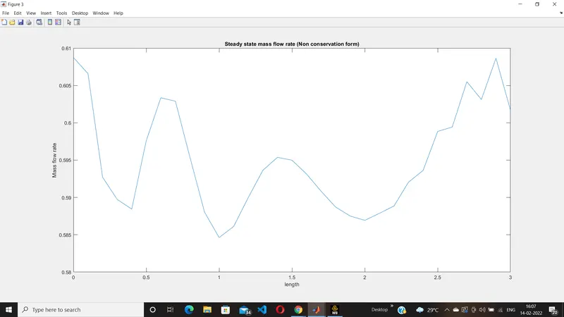
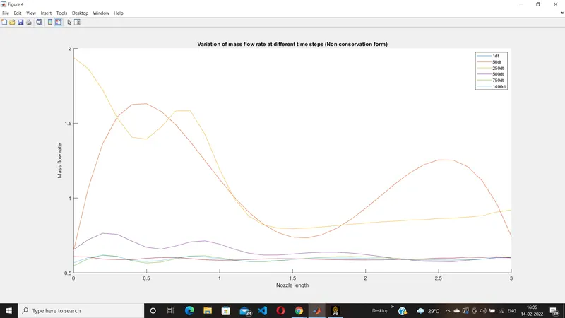
Here the mass flow rate is plotted as a function of non dimensional distance through the nozzle. Six different time steps are used in the graphs in time marching procedure.
As we can see from the graph after 250 time steps the plot starts to become stable
Conservation form:
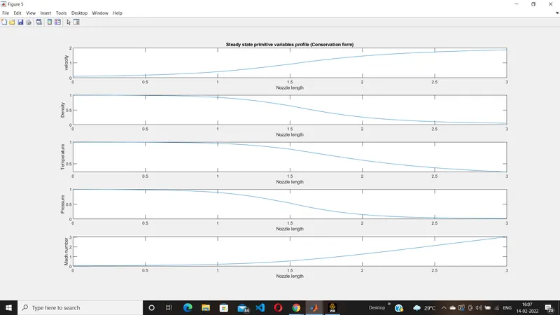
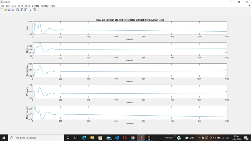
The above plots are drawn for each parameters such as Mach number,Density,Pressure,temperature for each time steps.
Initially, the values of all the parameters are very high and there are instabilities.And as the time step increases the plots become stable.
It is clearly seen that the values of conservative form have less oscillations than the non conservative form.
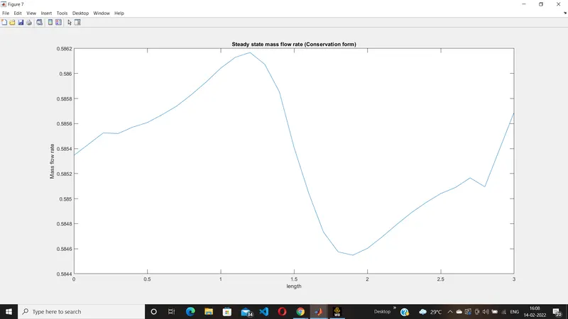
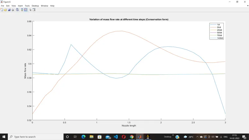
Here the mass flow rate is plotted as a function of non dimensional distance through the nozzle. Six different time steps are used in the graphs in time marching procedure.
As we can see from the graph after 250 time steps the plot starts to become stable
The variation in mass flow rate is less in the conservative form.
Comparison of mass flow rates between the two forms:
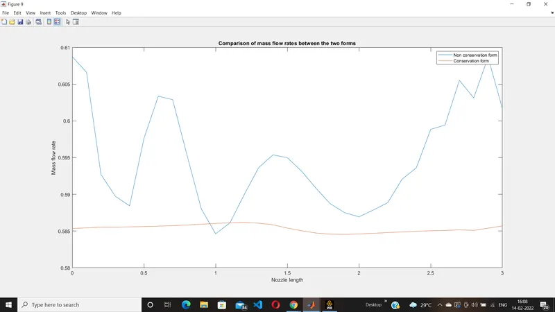
From the above plot we can conclude thatthe mass flow rate for conservative form along the length of nozzle shows the values are almost stable and there are very less instabilities.Whereas the mass flow rate in non conservative form is showing more instabilities in graph which say that the mass flow rate is at some points of nozzle is more(inflow & outflow boundaries) and becomes less at throat and varies.
Grid independance test:
Non conservation form:
When n = 31,
rho = 0.639
t = 0.836
p = 0.533
M = 0.999
When n = 61
rho = 0.638
t = 0.835
p = 0.532
M = 1
Conservation form:
When n = 31,
rho = 0.652
t = 0.841
p = 0.548
M = 0.978
When n = 61
rho = 0.639
t = 0.835
p = 0.534
M = 1
Analytical solution:
rho = 0.634
t = 0.833
p = 0.528
M = 1
Note that all the variables are in thier dimensionless forms.
From the above values the 61 grid points are closer to the analytical solution than the 31 grid points.So accuracy of solution increases with increase in grid points
Conclusion:
1. Mass flow rate is more stable in the conservative form.
2. Accuracy of the solution increases as the number of grid points increases.
3. The values of the primitive variables are same in both the forms.