Week 3.5 - Deriving 4th order approximation of a 2nd order derivative using Taylor Table method

1.Skewed right scheme:

'd^2u/dx^2` = (af(i)+bf(i+1)+cf(i+2)+df(i+3)+ef(i+4)+gf(i+5))/`dx^2`

Taylor table:

Term	f(i)	`Deltax*f'(i)`	`Deltax^2f''(i)`	`Deltax^3f'''(i)`	`Deltax^4f''''(i)`	`Deltax^5f'''''(i)`
f(i)	a	0	0	0	0	0
f(i+1)	b	b	b/2	b/6	b/24	b/120
f(i+2)	c	2c	4c/2	8c/2	16c/24	32c/120
f(i+3)	d	3d	9d/2	27d/6	81d/24	243d/120
f(i+4)	e	4e	16e/2	64e/6	256e/24	1024e/120
f(i+5)	g	5g	25g/2	125g/6	625g/24	3125g/120
`Deltax^2d^2u/dx^2`	0	0	1	0	0	0

a+b+c+d+e+g = 0 _______eqn 1

b+2c+3d+4e+5g = 0 ______eqn 2

b/2+4c/2+9d/2+16e/2+25g/2 = 1 __________eqn 3

b/6+8c/2+27d/6+64e/6+125g/6 = 0 _________eqn 4

b/24+16c/24+81d/24+256e/24+625g/24 = 0 _________eqn 5

b/120+32c/120+243d/120+1024e/120+3125g/120 = 0 ________eqn 6

These equations are written in a matrix from and are solved using Matrix inversion method.

No. of nodes ,N = 6

Order of derivative, Q = 2

Order of accuracy,P = N - Q = 6-2 = 4

Hence the skewed scheme is fourth order accurate

1.Central difference method:

'`^2u/dx^2` = (af(i-2)+bf(i-1)+cf(i)+df(i+1)+ef(i+2))/`dx^2`

Taylor table:

Term	f(i)	`Deltax*f'(i)`	`Deltax^2f''(i)`	`Deltax^3f'''(i)`	`Deltax^4f''''(i)`
f(i-2)	a	-2a	4a/2	-8a/6	16a/24
f(i-1)	b	-b	b/2	-b/6	b/24
f(i)	c	0	0	0	0
f(i+1)	d	e	d/2	d/6	d/24
f(i+2)	e	2e	4e/2	8e/6	16e/24
`Deltax^2d^2u/dx^2`	0	0	1	0	0

a+b+c+d+e = 0 _______eqn 1

-2a-b+d+2e = 0 ______eqn 2

4a/2+b/2+d/2+4e/2= 1 __________eqn 3

-8a/6-b/6+d/6+8e/6 = 0 _________eqn 4

16a/24+b/24+d/24+16e/24 = 0 _________eqn 5

These equations are written in a matrix from and are solved using Matrix inversion method.

1.Skewed left scheme:

'`^2u/dx^2` = (af(i)+bf(i-1)+cf(i-2)+df(i-3)+ef(i-4)+gf(i-5))/`dx^2`

Taylor table:

Term	f(i)	`Deltax*f'(i)`	`Deltax^2f''(i)`	`Deltax^3f'''(i)`	`Deltax^4f''''(i)`	`Deltax^5f'''''(i)`
f(i)	a	0	0	0	0	0
f(i-1)	b	-b	b/2	-b/6	b/24	-b/120
f(i-2)	c	-2c	4c/2	-8c/2	16c/24	-32c/120
f(i-3)	d	-3d	9d/2	-27d/6	81d/24	-243d/120
f(i-4)	e	-4e	16e/2	-64e/6	256e/24	-1024e/120
f(i-5)	g	-5g	25g/2	-125g/6	625g/24	-3125g/120
`Deltax^2d^2u/dx^2`	0	0	1	0	0	0

a+b+c+d+e+g = 0 _______eqn 1

-b-2c-3d-4e-5g = 0 ______eqn 2

b/2+4c/2+9d/2+16e/2+25g/2 = 1 __________eqn 3

-b/6-8c/2-27d/6-64e/6-125g/6 = 0 _________eqn 4

b/24+16c/24+81d/24+256e/24+625g/24 = 0 _________eqn 5

-b/120-32c/120-243d/120-1024e/120-3125g/120 = 0 ________eqn 6

These equations are written in a matrix from and are solved using Matrix inversion method.

No. of nodes ,N = 6

Order of derivative, Q = 2

Order of accuracy,P = N - Q = 6-2 = 4

Hence the skewed scheme is fourth order accurate.

Program:

for() loop is used so that the error values are calculated for a range of dx values

loglog(X,Y) plots x- and y-coordinates using a base 10 logarithmic scale on the x-axis and the y-axis.

clear all
close all
clc

%Given:
%f(x) = exp(x)*cos(x)
%Input variables
x = pi/3;
dx = linspace(pi,pi/30,100);

%Calling the functions
for i = 1:length(dx)
    skewed_right_error(i) = skewed_right_scheme(x,dx(i));
    central_diff_error(i) = central_diff_scheme(x,dx(i));
    skewed_left_error(i) = skewed_left_scheme(x,dx(i));
end

%Plotting the graph
figure(1)
loglog(dx,skewed_right_error,'-kd','MarkerFaceColor','r','MarkerSize',7,'linewidth',2)
hold on
loglog(dx,skewed_left_error,'-ko','MarkerFaceColor','g','MarkerSize',7,'linewidth',2)
hold on
loglog(dx,central_diff_error,'-ks','MarkerFaceColor','b','MarkerSize',7,'linewidth',2)
hold off
title('absolute error vs numerical error')
xlabel('dx')
ylabel('Error')
legend('skewed right error','skewed left error','central differencing' )

Function:

X = linsolve(A,B) solves the matrix equation AX = B, where B is a column vector.

abs() gives the magnitude.

function skewed_right_error = skewed_right_scheme(x,dx)
  

%Computing second order derivative for given f(x)
analytical_derivative = -2*exp(x)*sin(x);

%From taylor table:
A = [1 1 1 1 1 1;0 1 2 3 4 5;0 1/2 4/2 9/2 16/2 25/2;0 1/6 8/6 27/6 64/6 125/6;0 1/24 16/24 81/24 256/24 625/24;0 1/120 32/120 243/120 1024/120 3125/120]
B = [0;0;1;0;0;0];
X = linsolve(A,B);

a = X(1);
b = X(2);
c = X(3);
d = X(4);
e = X(5);
g = X(6);

%fourth order forward differencing
skewed_right_approx = ((a*exp(x)*cos(x))+(b*exp(x+dx)*cos(x+dx))+(c*exp(x+2*dx)*cos(x+2*dx))+(d*exp(x+3*dx)*cos(x+3*dx))+(e*exp(x+4*dx)*cos(x+4*dx))+(g*exp(x+5*dx)*cos(x+5*dx)))/(dx^2);


%Calculating error
skewed_right_error = abs(skewed_right_approx-analytical_derivative);

end

function central_diff_error = central_diff_scheme(x,dx)
  

%Computing second order derivative for given f(x)
analytical_derivative = -2*exp(x)*sin(x);

%From taylor table:
A = [1 1 1 1 1;-2 -1 0 1 2;4/2 1/2 0 1/2 4/2;-8/6 -1/6 0 1/6 8/6;16/24 1/24 0 1/24 16/24]
B = [0;0;1;0;0];
X = linsolve(A,B);

a = X(1);
b = X(2);
c = X(3);
d = X(4);
e = X(5);

%fourth order central differencing
central_diff_approx = ((a*exp(x-2*dx)*cos(x-2*dx))+(b*exp(x-dx)*cos(x-dx))+(c*exp(x)*cos(x))+(d*exp(x+dx)*cos(x+dx))+(e*exp(x+2*dx)*cos(x+2*dx)))/(dx^2);


%Calculating error
central_diff_error = abs(central_diff_approx-analytical_derivative);

end

function skewed_left_error = skewed_left_scheme(x,dx)
  

%Computing second order derivative for given f(x)
analytical_derivative = -2*exp(x)*sin(x);

%From taylor table:
A = [1 1 1 1 1 1;0 -1 -2 -3 -4 -5;0 1/2 4/2 9/2 16/2 25/2;0 -1/6 -8/6 -27/6 -64/6 -125/6;0 1/24 16/24 81/24 256/24 625/24;0 -1/120 -32/120 -243/120 -1024/120 -3125/120]
B = [0;0;1;0;0;0];
X = linsolve(A,B);

a = X(1);
b = X(2);
c = X(3);
d = X(4);
e = X(5);
g = X(6);

%fourth order  differencing
skewed_left_approx = ((a*exp(x)*cos(x))+(b*exp(x-dx)*cos(x-dx))+(c*exp(x-2*dx)*cos(x-2*dx))+(d*exp(x-3*dx)*cos(x-3*dx))+(e*exp(x-4*dx)*cos(x-4*dx))+(g*exp(x-5*dx)*cos(x-5*dx)))/(dx^2);


%Calculating error
skewed_left_error = abs(skewed_left_approx-analytical_derivative);

end

Plot:

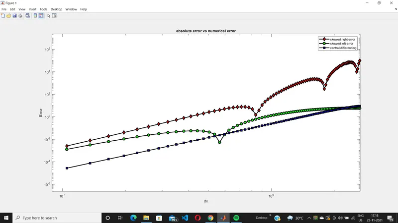
From the plot we can come to conclusion that the central difference method produces more accurate solutions than the skewed right adn skewed left schemes hence fewer errors.

Why a skewed scheme is useful? What can a skewed scheme do that a CD scheme cannot?

Eventhough the CD scheme provides accurate solutions it cannot be used at every situations. Say we need to calculate numerical approximations for a node on the corner or a boundary, we cannot always get the values on both sides of an ith point.So in this situtation we can use the skewed difference method as it only needs data of one side of the ith point.