Week 5.1 - Mid term project - Solving the steady and unsteady 2D heat conduction problem

Solving 2D Heat conduction equation:

The three dimensional heat equation with both time derivative and space derivative is given as follows:

`(delT)/(delt)+alpha((del^2T)/(delx^2)+(del^2T)/(dely^2)+(del^2T)/(delz^2))=0`

Since we are considering only 2D Heat equation (The above equation is solved for a thin plate),the dimesnions in the Z axis is neglected.Therefore the above equation is written as follows:

`(delT)/(delt)+alpha((del^2T)/(delx^2)+(del^2T)/(dely^2))=0`

This equation can be solved using two approaches:

1.Steady state equation:

Under steady state condition the rate of change of temperature is zero.

Steady state 2D equation:

`(del^2T)/(delx^2)+(del^2T)/(dely^2)=0`

2. Transient State equation:

Under transient state condition the temeperature changes with time,so the equation is :

`(delT)/(delt)+alpha((del^2T)/(delx^2)+(del^2T)/(dely^2))=0`

Assumptions:

Top Boundary = 600 K

Bottom Boundary = 900 K

Left Boundary = 400 K

Right Boundary = 800 K

Error = 9e9

Tolerance = 1e-4

Main program:

The functions to solve the 2D Heat conduction equation by different methods are called in the main program.

ones() is used to create an array containing only the number one.

clear all
close all  
clc

%Inputs

%No. of grid points
nx = 10;
ny = 10;


x = linspace(0,1,nx);
y = linspace(0,1,ny);
dx = x(2)-x(1);
dy = y(2)-y(1);
T = 450*ones(nx,ny);

%Boundary conditions
T(:,1) = 400;
T(:,end) = 800;
T(1,:) = 600;
T(end,:) = 900;

%Edge refining
T(1,1) = 0.5*(T(1,2)+T(2,1));
T(nx,1) = 0.5*(T(nx-1,1)+T(nx,2));
T(nx,ny) = 0.5*(T(nx,ny-1)+T(nx-1,ny));
T(1,ny) = 0.5*(T(1,ny-1)+T(2,ny));

%Assigning original values to T
T_old = T;
T_initial = T;
T_prev = T;

Method = input('Choose the method to be used');
error = 9e9;
tol = 1e-4;
conv = 9e9;

%Steady state 
if Method == 1
    %Calling the function for Jacobi method
    Jacobi_SS(nx,ny,dx,dy,T,T_old,error,tol)

    %Calling the function for Gauss Seidal method  
    Gauss_SS(nx,ny,dx,dy,T,T_old,error,tol)

    %Calling the function for Successive Over Realxation method
    SOR_SS(nx,ny,dx,dy,T,T_old,error,tol)
end


%Transient state 

%Solving implicitly
if Method == 2
     %Calling the function for Jacobi method
     Transient_implicit_jacobi(nx,ny,dx,dy,T,T_old,error,tol,T_initial,T_prev,conv)

     %Calling the function for Gauss Seidal method  
     Transient_implicit_gs(nx,ny,dx,dy,T,T_old,error,tol,T_initial,T_prev,conv)

     %Calling the function for Successive Over Realxation method 
     Transient_implicit_SOR(nx,ny,dx,dy,T,T_old,error,tol,T_initial,T_prev,conv)
end

%Solving explicitly
if Method == 3
     %Calling the function for Transient explicit method
     Transient_explicit(nx,ny,dx,dy,T,T_old,error,tol,T_initial,T_prev,conv)
end

Functions:

1. Steady State Analysis:

In steady state heat conduction the amount of heat entering any region of an object is equal to the amount of heat coming out.

`(del^2T)/(delx^2)+(del^2T)/(dely^2)=0`

By discretizing the equation above it becomes,

`T_p=1/k*[(T_L+T_R)/(Deltax^2)+(T_T+T_B)/(Deltay^2)]`

Value of K is,

`K=2((Deltax^2+Deltay^2)/(Deltax^2*Deltay^2))`

Substituting the values for `Deltax and Deltay` we get

`T_P=0.25*(T_L+T_R+T_T+T_B)`

Jacobi Method:

The Jacobi method is a method of solving a matrix equation on a matrix that has no zeros along its main diagonal . Each diagonal element is solved for, and an approximate value plugged in. The process is then iterated until it converges. This algorithm is a stripped-down version of the Jacobi transformation method of matrix diagnolization.

In Jacobi iteration method we use the values of the T_old for the next iteration.

function Jacobi_SS(nx,ny,dx,dy,T,T_old,error,tol)

%Initializing the number of iterations
Jacobi_iter = 0;

%Iteration solver
while(error>tol)
      for i = 2:nx-1;
          for j = 2:ny-1;

              T(i,j) = 0.25*(T_old(i+1,j)+T_old(i-1,j)+T_old(i,j-1)+T_old(i,j+1));
          end
      end
      %Finding error
      error = max(max(abs(T-T_old)));

      %Updating values
      T_old = T;

      %Incrementing
      Jacobi_iter = Jacobi_iter+1;

      %Plotting
      figure(1)
      contourf(flipud(T),'ShowText','on')
      colormap(jet)
      title(sprintf('Steady state Jacobi iterations = %d',Jacobi_iter));
      pause(0.005)
     
end
 colorbar
end

Gauss Seidal Method:

In numerical linear algebra, the Gauss–Seidel method, also known as the Liebmann method or the method of successive displacement, is an iterative method used to solve a system of linear equations.

In this iteration method the new values of T are used for the successive iterations.

function Gauss_SS(nx,ny,dx,dy,T,T_old,error,tol)

%Initializing the number of iterations
gs_iter = 0;

%Iteration solver
while(error>tol)
      for i = 2:nx-1;
          for j = 2:ny-1;
              T(i,j) = 0.25*(T_old(i+1,j)+T(i-1,j)+T(i,j-1)+T_old(i,j+1));
          end
      end
      %Calculating error
      error = max(max(abs(T-T_old)));

      %Updating values
      T_old = T;

      %Incrementing
      gs_iter = gs_iter+1;

      %Plotting
      figure(2)
      contourf(flipud(T),'ShowText','on')
      colormap(jet)
      title(sprintf('Steady state GS iterations = %d',gs_iter));
      pause(0.005)
     
end
 colorbar
end

Successive Over Relaxation Method(SOR):

In numerical linear algebra, the method of successive over-relaxation (SOR) is a variant of the Gauss Seidal method for solving a linear sysytem of equations, resulting in faster convergence. A similar method can be used for any slowly converging iterative process.

The formula is as follows:

`T_(i,j)=(1-omega)*T_(old_((i,j)))+omega*Tgs_(i,j)`

If omega > 1 it is said to be over realxed and if omega < 1 it is said to be under relaxed. Where omega is the scaling factor.

function SOR_SS(nx,ny,dx,dy,T,T_old,error,tol)

%Initializing
SOR_iter = 0;

omega = 1.5;

%Iterative solver
while(error>tol)
      for i = 2:nx-1;
          for j = 2:ny-1;

              T_gs(i,j) = 0.25*(T_old(i+1,j)+T(i-1,j)+T(i,j-1)+T_old(i,j+1));
              T(i,j) = (1-omega)*T_old(i,j)+omega*T_gs(i,j);
         
          end
      end
      %Calculating error
      error = max(max(abs(T-T_old)));

      %Updating values
      T_old = T;

      %Incrementing
      SOR_iter = SOR_iter+1;

      %Plotting
      figure(3)
      contourf(flipud(T),'ShowText','on')
      colormap(jet)
      title(sprintf('Steady state SOR iterations = %d',SOR_iter));
      pause(0.005)
     
end
 colorbar
end

2. Transient State Analysis:

Transient state 2D heat conduction equation is solved in both ways i.e explicitly and implicitly.Following is the 2D heat conduction equation.

`(delT)/(delt)+alpha((del^2T)/(delx^2)+(del^2T)/(dely^2))=0`

Solving implcitly:

Implicit approach is used in numerical analysis for obtaining numerical approximation to the solution of time dependent ordinary or partial differential equations as in required in computer simulations of a physical process.

Implicit methods find the solution by solving an equation involving both the current state of the system and the later one.

It is mathematically represented as Y(T+dt)

Discretizing the transient state equation we get (central differencing)

`(1+2k_1+2k_2)[T_p^n+k_1(T_L+T_R)^(n+1)+k_2(T_T+T_B)^(n+1)]`

Jacobi Method:

In Jacobi iteration method we use the values of the T_old for the next iteration.

function Transient_implicit_jacobi(nx,ny,dx,dy,T,T_old,error,tol,T_initial,T_prev,conv)

%Initializing iter values
Jacobi_iter = 0;
Jacobi_time_iter = 0;

%Variables
alpha = 0.015;
dt =1e-2;
k1 = alpha*dt/dx^2;
k2 = alpha*dt/dy^2;

%Time loop
while(conv>tol)
    %Space loop
    while(error>tol)
      for i = 2:nx-1;
              for j = 2:ny-1;
    
                  T(i,j) = (1+2*k1+2*k2)^-1*(T_prev(i,j)+k1*(T_old(i-1,j)+T_old(i+1,j))+k2*(T_old(i,j-1)+T_old(i,j+1)));

              end
      end
          %Calculating error
          error = max(max(abs(T-T_old)));

          %Updating T_old
          T_old = T;

          %Incrementing
          Jacobi_iter = Jacobi_iter+1;

          %Plotting
          figure(1)
          contourf(flipud(T),'ShowText','on')
          title(sprintf('Transient state implicit Jacobi iterations = %d Time iterations = %d',Jacobi_iter,Jacobi_time_iter));
          pause(0.005)
       
    end
          %Caculating convergence error
          conv = max(max(abs(T-T_prev)));

          %Updating T_prev
          T_prev = T;

          %Incrementing
          Jacobi_time_iter = Jacobi_time_iter+1;

          %Reinitializing error value
          error = 9e9;

end
colorbar
end

Gauss Seidal Method:

In this iteration method the new values of T are used for the successive iterations.

function Transient_implicit_gs(nx,ny,dx,dy,T,T_old,error,tol,T_initial,T_prev,conv)

%Initializing iter values
gs_iter = 0;
gs_time_iter = 0;

%Variables
alpha = 0.015;
dt =1e-2;
k1 = alpha*dt/dx^2;
k2 = alpha*dt/dy^2;

%Time loop
while(conv>tol) 
    %Space loop
    while(error>tol)
      for i = 2:nx-1;
              for j = 2:ny-1;
    
                  T(i,j) = (1+2*k1+2*k2)^-1*(T_prev(i,j)+k1*(T(i-1,j)+T_old(i+1,j))+k2*(T(i,j-1)+T_old(i,j+1)));

              end
      end
          %Calculating error 
          error = max(max(abs(T-T_old)));

          %Updating values
          T_old = T;

          %Incrementing
          gs_iter = gs_iter+1;

          %Plotting
          figure(2)
          contourf(flipud(T),'ShowText','on')
          title(sprintf('Transient state implicit Gauss seidal iterations = %d Time iterations = %d',gs_iter,gs_time_iter));
          pause(0.005)
         
    end
         %Calculating covergence error
         conv = max(max(abs(T-T_prev)));

         %Updating values
         T_prev = T;

         %Incrementing
         gs_time_iter = gs_time_iter+1;

         %Reinitializing error
         error = 9e9;

end
colorbar
end

Successive Over Relaxation(SOR):

The formula is as follows:

`T_(i,j)=(1-omega)*T_(old_((i,j)))+omega*Tgs_(i,j)`

If omega > 1 it is said to be over realxed and if omega < 1 it is said to be under relaxed. Where omega is the scaling factor.

function Transient_implicit_SOR(nx,ny,dx,dy,T,T_old,error,tol,T_initial,T_prev,conv)

%Initializing iter values
SOR_iter = 0;
SOR_time_iter = 0;

%Variables
alpha = 1.5;
omega = 1.5;
dt =1e-2;
k1 = alpha*dt/dx^2;
k2 = alpha*dt/dy^2;

%Time loop
while(conv>tol) 
    %Space loop
    while(error>tol)
      for i = 2:nx-1;
              for j = 2:ny-1;
    
                  T_GS(i,j) = (1+2*k1+2*k2)^-1*(T_prev(i,j)+k1*(T(i-1,j)+T_old(i+1,j))+k2*(T(i,j-1)+T_old(i,j+1)));
                  T(i,j) = (1-omega)*T_old(i,j)+omega*T_GS(i,j);
              end
      end
          %Calculating error value
          error = max(max(abs(T-T_old)));

          %Updating values
          T_old = T;

          %Incrementing
          SOR_iter = SOR_iter+1;

          %plotting
          figure(3)
          contourf(flipud(T),'ShowText','on')
          title(sprintf('Transient state implicit SOR iterations = %d Time iterations = %d',SOR_iter,SOR_time_iter));
          pause(0.005)
         
    end
      %Calculating convergence
      conv = max(max(abs(T-T_prev)));

      %Updating values
      T_prev = T;

      %Incrementing
      SOR_time_iter = SOR_time_iter+1;

      %Reinitialising error 
      error = 9e9;

end
colorbar
end

3. Transient State analysis:

Explicit Method:

Explicit approac is used in numerical analysis for obtaining approximations to the solutions of time-dependent ordinary or partial differential as required in computer simulations of a physical process.Explicit methods calculate the state of a system at a later time from the state of the system at the current time.

In this method, each differential equation approach contains only one unknown and can be solved explicitly for this one unknown using this method

function Transient_explicit(nx,ny,dx,dy,T,T_old,error,tol,T_initial,T_prev,conv)

%Initializing iter value
iter = 0;

%Varaiables
alpha = 0.015;
dt =1e-2;
k1 = alpha*dt/dx^2;
k2 = alpha*dt/dy^2;

while(conv>tol) 
      for i = 2:nx-1;
              for j = 2:ny-1;
    
                  T(i,j) = (1-2*k1-2*k2)*T_prev(i,j)+k1*(T_prev(i-1,j)+T_prev(i+1,j))+k2*(T_prev(i,j-1)+T_prev(i,j+1));

              end
      end
          %Calculating convergence    
          conv = max(max(abs(T-T_prev)));

          %Updating values
          T_prev = T;

          %Incrementing
          iter = iter+1;

          %Plotting
          contourf(flipud(T),'ShowText','on')
          title(sprintf('Transient state explicit iterations = %d',iter));
          pause(0.005)
          colorbar
           
end

end

Outputs:

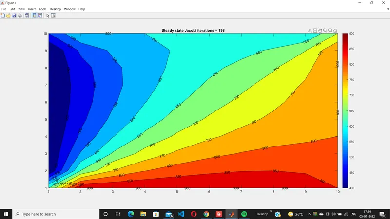
Steady state(Jacobi method):

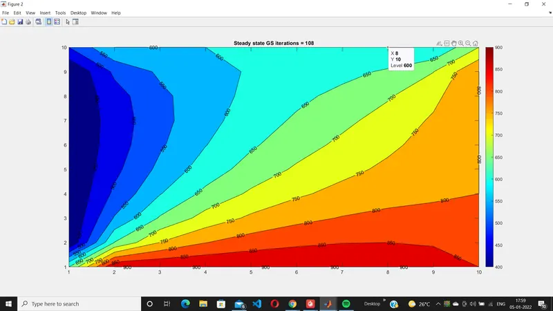
Steady state(Gauss Seidal method):

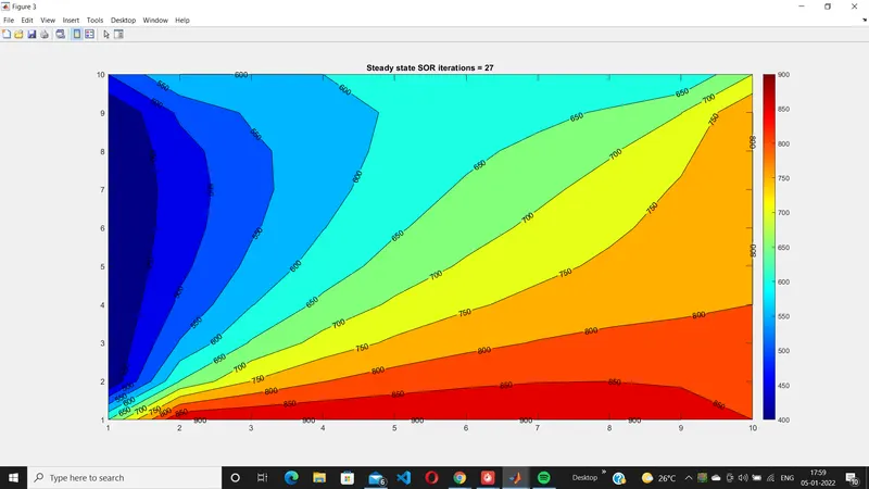
Steady state(Successive over relaxation):

Implicit approach:

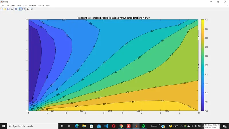
Transient state(Jacobi method):

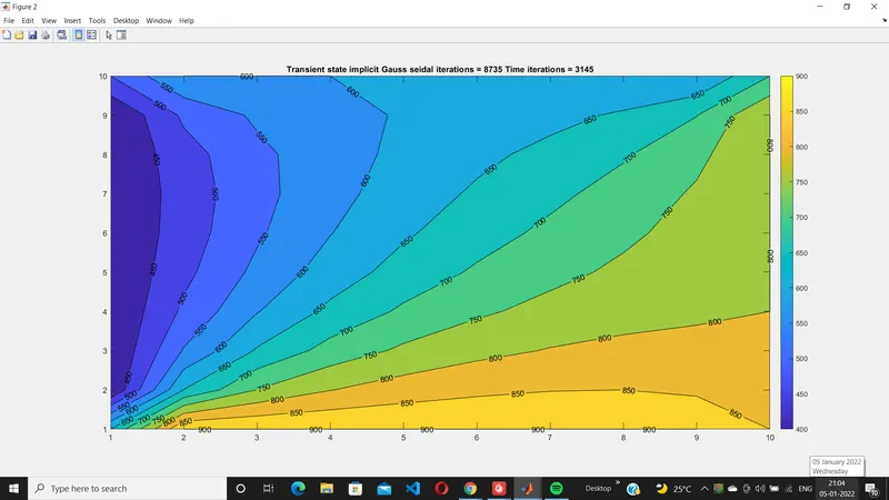
Transient state(Gauss Seidal method):

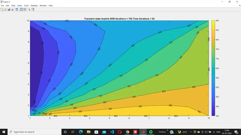
Transient state(Successive over relaxation):

Explicit approach:

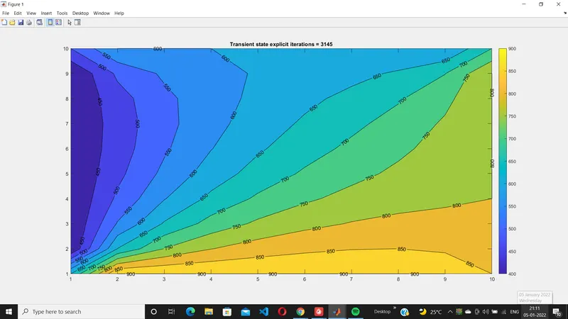
Transient state:

Conclusion:

1. In steady state equation the Jacobi method takes more number of iterations than the other two methods,whereas the SOR method yields results very quickly.So the most effecient method to solve the steady state equation is the SOR method.

2. For transient equations, explicit method yields results quickly when compared to the implicit approach.

When the transient state equation is solved implicitly SOR gives quick results.