Week 7 - Simulation of a 1D Super-sonic nozzle flow simulation using Macormack Method
Aim: Simulation of quasi 1D subsonic–supersonic nozzle flow using MacCormack method.
Objective: The objective of this project is to simulate an isentropic flow through a quasi 1D subsonic-supersonic nozzle using MacCormack method for conservation and non-conservation form of governing equations.
Theory: The subsonic-supersonic nozzle is also called as “convergent-divergent nozzle” or “de-laval nozzle”. The steady isentropic flow through a convergent-divergent nozzle is stated below,
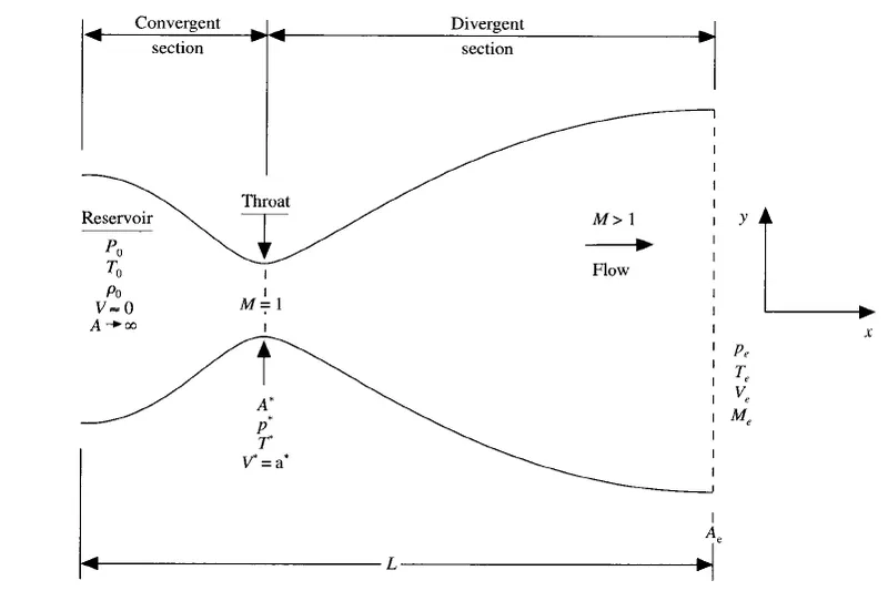
Fig(a): Schematic for subsonic-supersonic isentropic nozzle flow
So here, the flow at the inlet of the nozzle comes from a reservoir where pressure and temperature are denoted as by `p_0` and `T_0` respectively. The cross-sectional area of the reservoir is large (theoretically, `A->oo`), and hence velocity is very small (`V->0`). Thus, `p_0` and `T_0` are the stagnation values, or total pressure and total temperature, respectively. The flow expand isentropically to supersonic speeds at the nozzle exit, where the exit pressure, temperature, velocity and Mach number are denoted by `p_e, T_e,V_e and M_e` respectively. The flow is locally subsonic in the convergent section, sonic at the throat section and supersonic at the divergent section. The sonic flow (M=1) at the throat means that the local velocity at this location is equal to the local speed of sound. Using an asterisk to denote sonic flow values, we have the throat V=V*=a*. Similarly, the sonic flow values of pressure and temperature are denoted by `p_*` and `T_*` respectively.
Although the area of nozzle changes as a function of distance along the nozzle x and therefore in reality the flow field is two dimensional (xy space), we make the assumption that the flow properties vary only with x, this is the tantamount to assume uniform flow properties across any given cross-section. Such flow is defined as quasi-one dimensional flow.
Before, writing the governing equations in conservative and non-conservative form, we need to non-dimensionalize the primitive variables for removing the constraints of dimensions to analyse the numerical solution. It will certainly ease the method of analysis for a given problem.
Non-dimensional variables:
Temperature (T'): `T^'=T/T_0`
Density (`rho^'`): `rho^'=rho/rho_0`
Length (x’): `x^'=x/L`
Speed of the sound in the reservoir (`a_0`): `a_0=sqrt(gammaRT)`
Velocity (`V'`): `V^'=V/a_0`
Time(t’): `t'=t/(L/a_0)`
Area(A'): `A'=A/A^*`
Non-Conservative form:
1.Continuity Equation:
`(delrho^')/(delt^')=-rho^'*(delV^')/(delx^')-rho^'*V^'*(del(ln A^'))/(delx^')-V^'*(delrho^')/(delx^')`
2.Momentum Equation:
`(delV^')/(delt^')=-V^'*(delV^')/(delx^')-1/gamma*((delT^')/(delx^')+T^'/rho^'*(delrho^')/(delx^'))`
3.Energy Equation:
`(delT^')/(delt^')=-V^'*(delT^')/(delx^')-(gamma-1)*T^'*[(delV^')/(delx^')+V^'*(del(ln A^'))/(delx^']]`
Conservative form:
1.Continuity equation:
`(del(rho'A'))/(delt')+(del(rho'A'V'))/(delx')=0`
2.Momentum equation:
`(del(rho'A'V'))/(delt')+(del[rho'A'V'^2+(1/gamma)p'A'])/(delx')=(1/gamma)p'(delA')/(delx')`
3.Energy equation:
`(del[rho'((e')/(gamma-1)+gamma/2V'^2)A'])/(delt')+(del[rho'((e')/(gamma-1)+gamma/2V'^2)V'A'+p'A'V'])/(delx')=0`
Above equations are the non-dimensional conservative form of the continuity, momentum and energy equations for quasi-one-dimensional flow. Let us define the above equations in the simple generic form, which will be used in calculations instead of the above rigid and complex form. Element of the solutions vector U, the flux vector F, and the source term J as follows.
`U1=rho'A'`
`U2=rho'A'V'`
`U3=rho'((e')/(gamma-1)+gamma/2V'^2)A'`
`F1=rho'A'V'`
`F2=rho'A'V'^2+(1/gamma)p'A'`
`F3=rho'((e')/(gamma-1)+gamma/2V'^2)V'A'+p'A'V'`
`J2=1/gammap'(delA')/(delx')`
Before setting up numerical solution for conservative form, we must keep in mind that in the conservation form of the governing equations, the dependent variables (the variables for which we directly obtain numbers) are not primitive variables. In order to calculate the primitive variables, we need to decode the dependent variables and update our primitive variables in further steps.
MacCormack Method:
MacCormack’s method is an explicit finite-difference technique which is second order accurate in both space and time. MacCormack method generally uses three step approach (Predictor, Corrector & averaging) to calculate final numerical solution for an iteration. In predictor step, forward difference is taken for spatial derivatives whereas in corrector step rearward (backward) difference is taken for spatial derivatives. Furthermore, the solutions obtained from these two steps are averaged and final numerical solution is calculated for a single iteration.
Following is the step by step implementation of MacCormack method in non-conservative form of governing equations.
a) Predictor step:
1.Continuity Equation:
`((delrho)/(delt))_i^t=-rho_i^t*(V_(i+1)^t-V_i^t)/(Deltax)-rho_i^t*V_i^t*(lnA_(i+1)-lnA_i)/(Deltax)-V_i^t*(rho_(i+1)^t-rho_i^t)/(Deltax)` ………….(1)
2.Momentum Equation:
`((delrho)/(delt))_i^t=-V_i^t*(V_(i+1)^t-V_i^t)/(Deltat)-1/gamma((T_(i+1)^t-T_i^t)/(Deltax)+T_i^t/rho_i^t*(rho_(i+1)^t-rho_i^t)/(Deltat))` …........(2)
3.Energy Equation:
`((delT)/(delt))_i^t=-V_i^t*(T_(i+1)^t-V_i^t)/(Deltax)-(gamma-1)*T_i^t*((V_(i+1)^t-V_i^t)/(Deltax)+V_i^t*(lnA_(i+1)-lnA_i)/(Deltax))` ………..(3)
By solving this equation, we obtain the predicted values of ρ, V and T, denoted by the barred quantities, from
`(bar rho)_i^(t+Deltat)=rho_i^t+((delrho)/(delt))_i^t*Deltat` .........(4)
`(bar V)_i^(t+Deltat)=V_i^t+((delV)/(delt))_i^t*Deltat` .........(5)
`(bar T)_i^(t+Deltat)=T_i^t+((delT)/(delt))_i^t*Deltat` .........(6)
In equation 4 to 6 `rho_i^t`, `V_i^t`, and `T_i^t` are known values at time t. And the values for the time derivatives in equation 4 to 6 are supplied directly by the equations 1 to 3.
Moving to the corrector step, taking backward difference in spatial derivatives and using predicted barred quantities
(b) Corrector step:
1.Continuity Equation:
`(bar(delrho)/(delt))_i^(t+Deltat)=-bar rho_i^(t+Deltat)*(bar V_(i+1)^t-bar V_i^t)/(Deltax)-bar rho_i^t*bar V_i^t*(lnA_(i+1)-lnA_i)/(Deltax)-bar V_i^t*(bar rho_(i+1)^t-bar rho_i^t)/(Deltax)`………….(7)
2.Momentum Equation:
`(bar(delrho)/(delt))_i^t=-bar V_i^t*(bar V_(i+1)^t-bar V_i^t)/(Deltat)-1/gamma((bar T_(i+1)^t-bar T_i^t)/(Deltax)+bar T_i^t/bar rho_i^t*(bar rho_(i+1)^t-bar rho_i^t)/(Deltat))`…........(8)
3.Energy Equation:
`(bar(delT)/(delt))_i^t=-bar V_i^t*(bar T_(i+1)^t-bar V_i^t)/(Deltax)-(gamma-1)*bar T_i^t*((bar V_(i+1)^t-bar V_i^t)/(Deltax)+bar V_i^t*(lnA_(i+1)-lnA_i)/(Deltax))`………..(9)
After solving the barred quantities from corrected step, we can calculate the average time derivatives,
(c) Averaging time derivatives:
`((delrho)/(delt))_(av)=0.5*[((delrho)/(delt))_i^t+(bar (delrho)/(delt))_i^(t+Deltat)]`
`((delV)/(delt))_(av)=0.5*[((delV)/(delt))_i^t+(bar (delV)/(delt))_i^(t+Deltat)]`
`((delT)/(delt))_(av)=0.5*[((delT)/(delt))_i^t+(bar (delT)/(delt))_i^(t+Deltat)]`
Finally, we have the corrected values of the flow field variables at time (t+Δt), we get,
`rho_i^(t+Deltat)=rho_i^t+((delrho)/(delt))_(av)*Deltat`
`V_i^(t+Deltat)=V_i^t+((delV)/(delt))_(av)*Deltat`
`T_i^(t+Deltat)=T_i^t+((delT)/(delt))_(av)*Deltat`
These variables are non-dimensional values and constitute our second eschelon of equations i.e the finite difference expressions of the governing equations in a form that pertains to MacCormack technique.
Note: Similarly, implement these steps for conservative form of the governing equations.
Initial and Boundary conditions:
To start the time marching calculations, we must stipulate initial conditions for ρ, T and V as a function of x; that is, we must set up values of ρ, T and V at time t=0.
Non-conservative form:
Initial condition:
`rho=1-0.3146x`
`T=1-0.2314x`
`V=(0.1+1.09x)*T^0.5`
Boundary conditions:
In our case, we are having a subsonic flow in the convergent section (M<1), choked flow at the throat section (M=1) and supersonic outflow in the divergent section (M>1). So by using method of characteristics for an unsteady, one dimensional flow we can precisely allot inflow and outflow boundary condition and can identify which quantities to state at the boundaries.
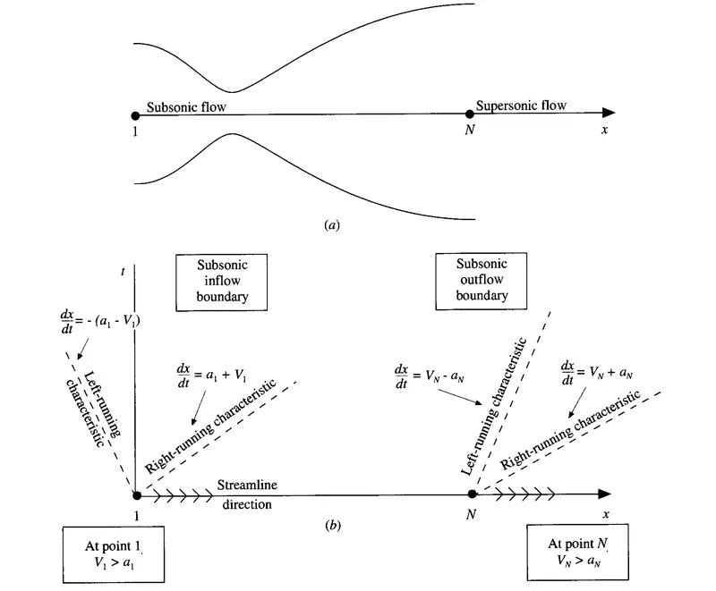
Fig (b) : Study of boundary conditions: subsonic inflow and supersonic outflow
What does these characteristics curve and streamline direction tell us?
- If any characteristic line is entering into the domain, implies that the value of one dependent flow field variable must be specified at that boundary.
- However, if any characteristic line is exiting the domain, implies that the value of the another dependent flow field variable must be allowed to float at that boundary i.e. it must be calculated in steps of time as function time wise solution of the flow field.
- Similarly, if streamline flows into the domain then specify third dependent flow field variable and if streamline flows out of the domain then third dependent flow field variable must be allowed to float.
In our case, at i = 1(inlet), we have primitive variables like ρ, A, V and T. So which variables must be taken for initial and boundary conditions? Here, we know the ρ and T at node 1 are equal to the reservoir's ρ and T which is assumed to be ρ=1 and T = 1, so it becomes,
Inflow boundary condition:
ρ(1)=1 and T(1)=1 (Since it is Dirichlet boundary condition)
However, velocity and area tends to infinity, so for velocity, we need to calculate it from the information obtained from inner nodes,
V(1)=2⋅V(2)-V(3) (It is Neumann boundary condition)
Outflow boundary condition:
At the outflow boundary condition (Node =n), as we can see that, both the characteristics lines are out of the domain and streamline also flows out of the domain. This is because, at the outflow condition, the flow is supersonic (M>1), which is certainly greater than the speed of sound. So in this condition, information transport is very fast. Therefore, there are no flow field variables which require their values to be stipulated at the supersonic outflow boundary; all variables must be allowed to float at this boundary.
ρ(n)=2⋅ρ(n-1)-ρ(n-2)
V(n)=2⋅V(n-1)-V(n-2)
T(n)=2⋅T(n-1)-T(n-2)
The supersonic outflow boundary is purely Neumann boundary condition, which is extrapolating the boundary nodes using the information from inner nodes.
Conservative form:
In conservative form, we will initialize the nozzle profile rationally. As in conservative form, seen above from the governing equations, we have solution vectors, flux terms and a source term. So it is the prior matter of concern to state initial and boundary conditions in those terms rather than that of primitive variables.
Initial conditions:
These variations are slightly more realistic than those assumed in the nozzle shape and initial conditions in non-conservative form of governing equations discussed above. This is an anticipation that the stability behaviour of the finite-difference formulation using the conservation form of the governing equations might be slightly more sensitive, and therefore it is useful to start with more improved initial conditions than those discussed above in non-conservative form.
Assumptions for initial profile of the nozzle:
- For 0≤x′≤0.5
ρ'=1
T′=1
- For 0.5≤x′≤1.5
ρ′=1.0-0.366(x′-0.5)
T′=1.0-0.167(x′-0.5)
- For 1.5≤x′≤3.5
ρ′=0.634-0.3879(x′-1.5)
T′=0.833-0.3507(x′-1.5)
Before stating the initial conditions in terms of solution vectors, we need to initialize velocity (V'). We have one of the dependent variable in our governing equation as U2, which is physically local mass flow; that is U2=ρ'A'V'. Therefore, for the initial conditions only; let us assume a constant mass flow through the nozzle and calculate V` as,
V'=U2/ρ'A'=0.59/ρ'A'
Note: The value 0.59 is chosen for U2, because it is close to exact analytical value of the steady-state mass flow (which is for this case is 0.579)
Therefore, the initial condition for V′ as a function of x′ is obtained by substituting the ρ′ and A′ variation. Finally, the initial conditions for U1, U2, U3 are obtained by substituting the above variations for ρ′, T′ and V′ into the definitions discussed above.
U1=ρ'A'
U2=ρ'A'V'
U3=`rho'((e')/(gamma-1)+gamma/2V'^2)A'`
where, e′=T′ Certainly, for the initial conditions described above, V′ is calculated such that U2=ρ'A'V'=0.59
Boundary conditions:
In conservative form, by referring fig (b) and absorbing the same method of characteristics approach we can allot boundary conditions for inflow and outflow boundary conditions. However, in this case, the boundary conditions will be in terms of solution vectors. Similarly as discussed above, at the subsonic inflow (M<1), we need to specify two quantities at the initial node, where we have ρ′, A′ and U2=ρ'A'V'=0.59 (Mass flow rate) specified and one quantity will be allowed to float by referring left hand characteristic line. However, at the supersonic outflow (M>1), the information is travelling exceeds the speed of sound, hence it is irrational to specify outflow boundary condition. Therefore, all the dependent variables are allowed to float and they will be calculated in steps of time as a function time-wise solution of the flow field.
Inflow boundary condition:
The inflow boundary condition can be given as,
U1=ρ'(1)*A'(1) (Dirichlet boundary condition)
U2=2*U2(2)-U2(3)
V(1)=U2(1)/U1(1)
Note: This velocity at the first node will be substituted below in calculating U3
U3=`U1(1)[(T(1))/(gamma-1)+gamma/2(V'(1))^2]` (Neumann boundary condition)
Outflow boundary condition:
All the dependent variables will be allowed to float. Hence, the outflow boundary can be given as,
U1(n)=2⋅U1(n−1)−U1(n−2) (Neumann boundary condition)
U2(n)=2⋅U2(n−1)−U2(n−2) (Neumann boundary condition)
U3(n)=2⋅U3(n−1)−U3(n−2) (Neumann boundary condition)
Time step calculation:
The governing system of equations is hyperbolic with respect to time. So there is stability constraint on this system which is known as Courant-Friedrich-Lewy (CFL) condition. The Courant number is a simple stability analysis of a linear hyperbolic equations that gives result C≤1 for an explicit numerical solution to be stable.
CFL condition can be given as,
CFL condition = (any quantity)*(time-step with which information would travel)/(element step size)
So, in our case, the quantity which is going to travel is velocity, or in other sense velocity is the quantity which will be travelling with certain time from one node to other. So here velocity of the fluid at a point in the flow is coupled with local speed of sound. The quantity can be expressed to be as a+V'
CFL = `(a+V')*(Deltat)/(Deltax)`
We will assume the Courant number as C = 0.5, accordingly will calculate the △t. In addition to it, we will calculate `(Deltat)_i^t` at all the grid points, i = 1 to i = n, and then we'll choose the minimum value of △t in our calculations.
After considering all these governing equations and their respective pre-requisites to solve the problem, then we will move towards to the MATLAB code for execution.
Main MATLAB code:
close all
clear all
clc

% Defining inputs
L=3;                        % length of domain
n=31;                       % Total number of nodes in x-dimension
x=linspace(0,L,n);          % x-dimension grids
dx=x(2)-x(1);               % Elemental step size
gamma=1.4;                  % Specific heat capacity of air
a=1+2.2*(x-1.5).^2;         % Area of the nozzle
C=0.5;                      % CFL number
nt=1400;                    % Total time steps
time_step=linspace(1,nt,nt);% Dummy variable of total number of time steps

% Steady state analytical mass flow distribution
mflow_an=0.579*ones(n);

% For better representation 1 & 2 suffix for non-conservative &
% conservative function's variable respectively
% Calling non-conservative function
[rho1,v1,t1,p1,mach1,mflow1,rho_th1,v_th1,t_th1,p_th1,mach_th1]=non_conservative(x,nt,n,dx,gamma,a,mflow_an);
% Calling conservative function
[rho2,v2,t2,p2,mach2,mflow2,rho_th2,v_th2,t_th2,p_th2,mach_th2]=conservative(x,nt,n,dx,gamma,a,mflow_an);

% Plot variation of flow parameter inside the nozzle
    figure(3)
    subplot(4,1,1)
    plot(x,rho1,x,rho2,'linewidth',2)
    xlabel('Non-dimensional distance through the nozzle(x)')
    ylabel('Density(rho)')
    title('Steady-state distribution of primitive variables(Density) inside the nozzle')
    legend('Non-conservative form','Conservative form')
    grid on

    subplot(4,1,2)
    plot(x,t1,x,t2,'linewidth',2)
    xlabel('Non-dimensional distance through the nozzle(x)');
    ylabel('Temperature(t)');
    title('Steady-state distribution of primitive variables(Temperature) inside the nozzle')
    legend('Non-conservative form','Conservative form')
    grid on

    subplot(4,1,3)
    plot(x,p1,x,p2,'linewidth',2)
    xlabel('Non-dimensional distance through the nozzle(x)');
    ylabel('Pressure(p)');
    title('Non-dimensional Pressure variation(p) along x at 1400th timestep')
    legend('Non-conservative form','Conservative form')
    grid on

    subplot(4,1,4)
    plot(x,mach1,x,mach2,'linewidth',2)
    xlabel('Non-dimensional distance through the nozzle(x)');
    ylabel('Mach number(M)');
    title('Non-dimensional Mach number variation(M) along x at 1400th timestep')
    legend('Non-conservative form','Conservative form','location','north')
    grid on

    % Comparison of timewie variation of flow field variables at the throat
    % section
    figure(4)
    subplot(4,1,1)
    plot(time_step,rho_th1,time_step,rho_th2,'linewidth',2)
    xlabel('Number of time steps')
    ylabel('Density(rho)')
    title('Time wise variation of flow variables at throat section(Density)')
    legend('Non-conservative form','Conservative form')
    grid on

    subplot(4,1,2)
    plot(time_step,t_th1,time_step,t_th2,'linewidth',2)
    xlabel('Number of time steps')
    ylabel('Temperature(t)')
    title('Time wise variation of flow variables at throat section(Temperature)')
    legend('Non-conservative form','Conservative form')
    grid on

    subplot(4,1,3)
    plot(time_step,p_th1,time_step,p_th2,'linewidth',2)
    xlabel('Number of time steps')
    ylabel('Pressure(p)')
    title('Time wise variation of flow variables at throat section(Pressure)')
    legend('Non-conservative form','Conservative form')
    grid on

    subplot(4,1,4)
    plot(time_step,mach_th1,time_step,mach_th2,'linewidth',2)
    xlabel('Number of time steps')
    ylabel('Mach number(M)')
    title('Time wise variation of flow variables at throat section(Mach number)')
    legend('Non-conservative form','Conservative form')
    grid on

    % Plot steady state mass flow variations obtained with non-conservation
    % form of the governing equations
    figure(5)
    plot(x,mflow1,x,mflow2,x,mflow_an,'linewidth',2)
    xlabel('Non-dimensional distance through the nozzle(x)')
    ylabel('Non-dimensional mass flow rate (rho*v*a)')
    title('Comparison of mass flow rate variation')
    legend('Non-conservative form','Conservative form','Exact analytical solution','location','north')
Function code for Non-conservative form:
function[rho1,v1,t1,p1,mach1,mflow1,rho_th1,v_th1,t_th1,p_th1,mach_th1]=non_conservative(x,nt,n,dx,gamma,a,mflow_an)
% Calculate initial profiles
rho1=1-0.3146*x;            % density
t1=1-0.2314*x;              % t=temperature
v1=(0.1+1.09*x).*t1.^0.5;    % velocity

% Outer time loop
for k=1:nt
    rho_old=rho1;
    v_old=v1;
    t_old=t1;

    % Adaptive time step(To calculate min time step using CFL condition)
    dt=0.0201;     % According to J D Anderson book

    % Predictor Method
    for j=2:n-1
        % drho_dt_p=-rho(j)*(v(j+1)-v(j))/dx-rho(j)*v(j)*(log(a(j+1))-log(a(j)))/dx-v(j)*(rho(j+1)-rho(j))/dx;
        dvdx=(v1(j+1)-v1(j))/dx;
        drhodx=(rho1(j+1)-rho1(j))/dx;
        dtdx=(t1(j+1)-t1(j))/dx;
        dlogadx=(log(a(j+1))-log(a(j)))/dx;

        % Continuity equation
        drhodt_p(j)=-rho1(j)*dvdx-rho1(j)*v1(j)*dlogadx-v1(j)*drhodx;

        % Momentum equation
        dvdt_p(j)=-v1(j)*dvdx-(1/gamma)*(dtdx+(t1(j)/rho1(j))*drhodx);

        % Energy equation
        dtdt_p(j)=-v1(j)*dtdx-(gamma-1)*t1(j)*(dvdx+v1(j)*dlogadx);

        % solution update
        rho1(j)=rho1(j)+drhodt_p(j)*dt;
        v1(j)=v1(j)+dvdt_p(j)*dt;
        t1(j)=t1(j)+dtdt_p(j)*dt;
    end

    % Corrector Method
    for j=2:n-1
        % drho_dt_c=-rho(j)*(v(j)-v(j-1))/dx-rho(j)*v(j)*(log(a(j))-log(a(j-1)))/dx-v(j)*(rho(j)-rho(j-1))/dx;
        dvdx=(v1(j)-v1(j-1))/dx;
        drhodx=(rho1(j)-rho1(j-1))/dx;
        dtdx=(t1(j)-t1(j-1))/dx;
        dlogadx=(log(a(j))-log(a(j-1)))/dx;

        % Continuity equation
        drhodt_c(j)=-rho1(j)*dvdx-rho1(j)*v1(j)*dlogadx-v1(j)*drhodx;

        % Momentum equation
        dvdt_c(j)=-v1(j)*dvdx-(1/gamma)*(dtdx+(t1(j)/rho1(j))*drhodx);

        % Energy equation
        dtdt_c(j)=-v1(j)*dtdx-(gamma-1)*t1(j)*(dvdx+v1(j)*dlogadx);
    end

    % Compute the average time derivative
    drhodt=0.5*(drhodt_p+drhodt_c);
    dvdt=0.5*(dvdt_p+dvdt_c);
    dtdt=0.5*(dtdt_p+dtdt_c);

    % Final solution update
    for j=2:n-1
        rho1(j)=rho_old(j)+drhodt(j)*dt;
        v1(j)=v_old(j)+dvdt(j)*dt;
        t1(j)=t_old(j)+dtdt(j)*dt;
        % Calculate mass flow rate
        mflow1(j)=rho1(j)*a(j)*v1(j);
    end

    % Apply the boundary conditions
    % Inlet
    rho1(1)=1;             % Dirichlet BC
    t1(1)=1;               % Dirichlet BC
    v1(1)=2*v1(2)-v1(3);     % Nuemann BC

    % Outlet
    v1(n)=2*v1(n-1)-v1(n-2);         % Nuemann BC
    rho1(n)=2*rho1(n-1)-rho1(n-2);   % Nuemann BC
    t1(n)=2*t1(n-1)-t1(n-2);         % Nuemann BC

    % Calculating other variables
    mflow1=rho1.*a.*v1;
    mach1=v1./(t1.^0.5);
    p1=rho1.*t1;

    % Calculating throat variable
    rho_th1(k)=rho1(16);
    t_th1(k)=t1(16);
    v_th1(k)=v1(16);
    p_th1(k)=p1(16);
    mach_th1(k)=mach1(16);

    % Plotting time-wise variation of mass flow rate
    figure(1)
    if k==50
        plot(x,mflow1,'r','linewidth',2)
        hold on
    elseif k==200
        plot(x,mflow1,'b','linewidth',2)
    elseif k==400
        plot(x,mflow1,'m','linewidth',2)
    elseif k==700
        plot(x,mflow1,'g','linewidth',2)
    elseif k==1400
        plot(x,mflow1,'y','linewidth',2)
        plot(x,mflow_an,':','linewidth',2)
        hold off
    end
end
    xlabel('Non-dimensional distance through nozzle(x)')
    ylabel('Non-dimensional mass flow rate(mflow)')
    title('Non-dimensional mass flow rate (Non-conservative form) along x at different time steps')
    legend('50 time-step','200 time-step','400 time-step','700 time-step','1400 time-step','Exact analytical solution')
end
Function code for Conservative form:
function[rho2,v2,t2,p2,mach2,mflow2,rho_th2,v_th2,t_th2,p_th2,mach_th2]=conservative(x,nt,n,dx,gamma,a,mflow_an)
% Initial condition
for i=1:n
    if (x(i)>=0 && x(i)<=0.5)
        rho2(i)=1;
        t2(i)=1;      % t=temperature
    elseif (x(i)>0.5 && x(i)<=1.5)
        rho2(i)=1-0.366*(x(i)-0.5);
        t2(i)=1-0.167*(x(i)-0.5);
    elseif (x(i)>1.5 && x(i)<=3.5)
        rho2(i)=0.634-0.3879*(x(i)-1.5);
        t2(i)=0.833-0.3507*(x(i)-1.5);
    end
end
% velocity
v2=0.59./(rho2.*a);

% Solution variables initialization
U1=rho2.*a;
U2=rho2.*a.*v2;
U3=rho2.*((t2./(gamma-1))+(gamma/2).*v2.^2).*a;

for k=1:nt
    U1_old=U1;
    U2_old=U2;
    U3_old=U3;

    rho_old=rho2;
    v_old=v2;
    t_old=t2;

    % Adaptive time step method
    dt=0.0267;     % According to J D Aderson book

    % Steady state analytical mass flow distribution
    mflow_an=0.579*ones(n);

    % Initialization of flux
    F1=U2;
    F2=(U2.^2./U1)+(((gamma-1)/gamma)*(U3-(gamma/2)*(U2.^2./U1)));
    F3=(gamma*U2.*U3./U1)-((gamma*(gamma-1)/2)*(U2.^3./U1.^2));
    % Predictor Method
    for j=2:n-1
        % Source Term
        J2=(1/gamma)*rho2.*t2*((a(j+1)-a(j))/dx);
        % Continuity Equation
        dU1dt_p(j)=-((F1(j+1)-F1(j))/dx);
        % Momentum Equation
        dU2dt_p(j)=-((F2(j+1)-F2(j))/dx)+J2(j);
        %Energy Equation
        dU3dt_p(j)=-((F3(j+1)-F3(j))/dx);
        % solution updates
        U1(j)=U1(j)+dU1dt_p(j)*dt;
        U2(j)=U2(j)+dU2dt_p(j)*dt;
        U3(j)=U3(j)+dU3dt_p(j)*dt;

    end
    % updated primitive variables using predicted values
    rho2=U1./a;
    v2=U2./U1;
    t2=(gamma-1)*((U3./U1)-(gamma/2)*v2.^2);
    p2=rho2.*t2;

    % Recompute the flux variable using predicted value
    F1=U2;
    F2=(U2.^2./U1)+(((gamma-1)/gamma)*(U3-(gamma/2)*(U2.^2./U1)));
    F3=(gamma*U2.*U3./U1)-((gamma*(gamma-1)/2)*(U2.^3./U1.^2));

    % Corrector Method
    for j=2:n-1
        % Source Term
        J2=(1/gamma)*rho2.*t2*((a(j)-a(j-1))/dx);
        % Continuity equation
        dU1dt_c(j)=-((F1(j)-F1(j-1))/dx);
        % Momentum equation
        dU2dt_c(j)=-((F2(j)-F2(j-1))/dx)+J2(j);
        % Energy equation
        dU3dt_c(j)=-((F3(j)-F3(j-1))/dx);
    end

    % Averages of predictor-corrector step time derivative
    dU1dt_avg=0.5*(dU1dt_p+dU1dt_c);
    dU2dt_avg=0.5*(dU2dt_p+dU2dt_c);
    dU3dt_avg=0.5*(dU3dt_p+dU3dt_c);

    % Final solution update
    for j=2:n-1
        U1(j)=U1_old(j)+dU1dt_avg(j)*dt;
        U2(j)=U2_old(j)+dU2dt_avg(j)*dt;
        U3(j)=U3_old(j)+dU3dt_avg(j)*dt;
        % Calculate mass flow rate
        mflow2(j)=rho2(j)*a(j)*v2(j);
    end

    % Apply Boundary conditions
    % Inlet(subsonic inflow)
    U1(1)=a(1)*rho2(1);                     % Dirichlet BC
    U2(1)=2*U2(2)-U2(3);                   % Neumann BC
    U3(1)=U1(1)*((t2(1)/(gamma-1))+((gamma/2)*(U2(1)/U1(1))^2)); %Neumann BC
    % outlet(supersonic outflow)
    U1(n)=2*U1(n-1)-U1(n-2);          % Neumann BC
    U2(n)=2*U2(n-1)-U2(n-2);          % Neumann BC
    U3(n)=2*U3(n-1)-U3(n-2);          % Neumann BC

    % Update primitive variable
    rho2=U1./a;
    v2=U2./U1;
    t2=(gamma-1)*((U3./U1)-(gamma/2)*v2.^2);

    % Calculating other variables
    mflow2=rho2.*a.*v2;
    mach2=v2./(t2.^0.5);
    p2=rho2.*t2;

    % Calculating throat variable
    rho_th2(k)=rho2(16);
    t_th2(k)=t2(16);
    v_th2(k)=v2(16);
    p_th2(k)=p2(16);
    mach_th2(k)=mach2(16);

    % Plotting time-wise variation of mass flow rate
    figure(2)
    if k==50
        plot(x,mflow2,'r','linewidth',2)
        hold on
    elseif k==200
        plot(x,mflow2,'b','linewidth',2)
    elseif k==400
        plot(x,mflow2,'m','linewidth',2)
    elseif k==700
        plot(x,mflow2,'g','linewidth',2)
    elseif k==1400
        plot(x,mflow2,'y','linewidth',2)
        plot(x,mflow_an,':','linewidth',2)
        hold off
    end
end
    xlabel('Non-dimensional distance through nozzle(x)')
    ylabel('Non-dimensional mass flow rate(mflow)')
    title('Non-dimensional mass flow rate (Conservative form) along x at different time steps')
    legend('50 time-step','200 time-step','400 time-step','700 time-step','1400 time-step','Exact analytical solution','location','north')
end
Results and discussions:
Plots:
1.Steady state distribution of primitive variables inside the nozzle:
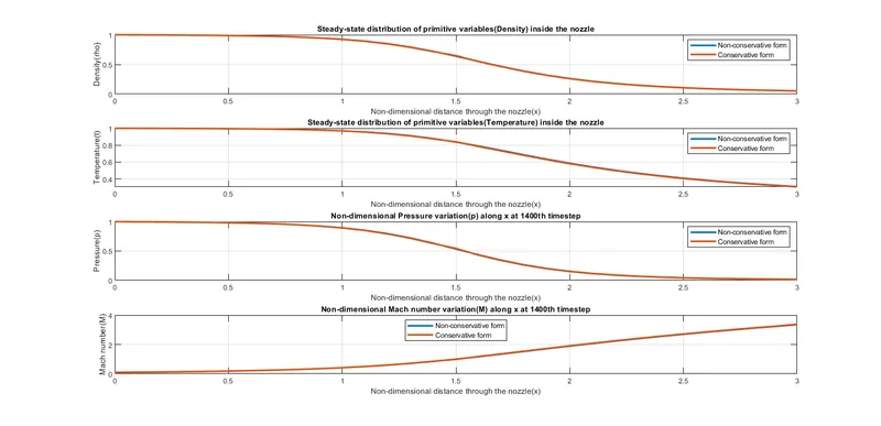
Discussion:
The steady state distribution inside the nozzle is resulted as above. After 1400 time steps, the numerically calculated primitive variables are converged to the exact analytical solution. The variations along the non-dimensional distance of the nozzle is explicitly resulted. Initially some of the primitive variables were set to initial condition and other were allowed to float as a part of inflow subsonic boundary condition. At n = 1, non-dimensional pressure or pressure ratio (`p/p_0`) of the fluid element was set to 1 (reservoir end), then as a part of numerical explicit scheme (MacCormack method), the pressure variations were calculated as function of time along the nozzle. There is decrease in the pressure as the flow changes from subsonic (convergent s/c, M<1) to sonic (throat s/c, M=1) state and similarly from sonic (throat s/c, M=1) to supersonic (divergent s/c, M>1) state. Similar is the case for density and temperature. The pressure difference present inside the system and in the surronding is responsible for the fluid flow. This pressure difference (reservoir and exit/surronding) gradually decreases as a function of time and length of the nozzle as the fluid travels towards the exit of the divergent section. Conversely, velocity of the fluid will increase travelling through convergent (subsonic, a-V), throat(sonic, V = a) and divergent section(supersonic, V+a). Similarly, as the velocity increases, Mach number will increase accordingly as function of length of the nozzle. Both conservative and non-conservative form of the governing equations show steady state results and show similar results at the macroscopic level.
2.Time-wise variations of the primitive variables:
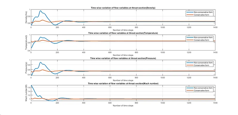
Discussion:
The variation of all the primitive variables at the throat section are resulted as function of time. The results are changing continuously as the time advances from an initial state (t=0). The MacCormack method is converging numerical results with each iteration in fast and robust manner. As we know, the throat section is responsible for increasing the velocity of the fluid element to a sonic state. It is prime reference for our calculations to compare results at the throat section with exact analytical solution at throat. So it neccessary to plot variations of the primitive variables as a part of time marching process. When using nodes as 31, there is very minute difference between variations of the primitive variables at the end of time (1400 time-steps) using conservative and non-conservative form. However, there is very slight and negligible difference in between both the curves obtain steady state at the end of 1400 time steps (i.e. numerically converged to exact analytical solution).
3.Variation of mass flow distribution inside the nozzle at different time-steps during the time-marching process:
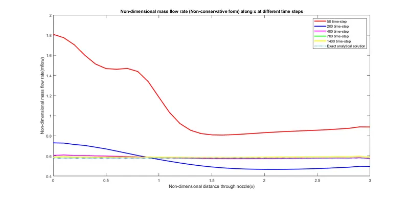
Non-conservative form:
3.2 Conservative form:
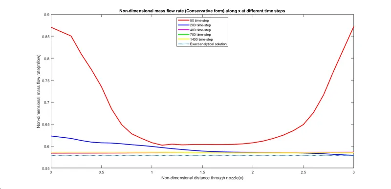
Discussion:
In these above plots, the mass flow distribution has resulted as function of advancement in time-step. Irrespective of the form of governing equation used, the mass flow distribution at first 50 time-step shows drastic variation. As the time step progresses, the mass flow distribution variation decreases and somewhat linearizes eventually. This is because the numerical result takes time to converge to the exact analytical solution. In addition to it, the conservative form has less variations among the curves as compared to non-conservative form. This is because we provided improved initial condition for conservative form. Due to this, the initial condition was defined close to steady state solution which refined the process flow. So at 1400th time step, both the form of numerical solution (Conservative and non-conservative) converged to the exact analytical solution numerically.
4.Comparison of normalized mass flow rate distributions of both forms:
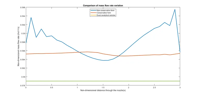
Discussion:
The comparison of mass flow distribution is plotted against the non-dimensional nozzle distance. By observing the above plot, we can state that the mass flow distribution predicted by the conservative form of equations shows good results than that of the non-conservative form. This is because of some inferences from the resulted graph. The conservation form gives a distribution that is much closer to being a constant. However, the non-conservative form shows significant variation and oscillations at the inflow and outflow boundaries. The reason behind conservation form to yield better results is that mass flow is one of the dependent variables in the equations, which mean that the mass flow is a primary result of the equations. In contrast to it, the dependent variables in the non-conservation form of the equations are the primitive variables, and the mass flow is obtained only as a secondary result.
Conclusion:
In summary, for the given flow problem, we cannot establish an assertion that which form of equation (conservation or non-conservation) has superiority over the other form. In essence, from our previous discussions, we can only make the following observations:
- The conservation form yields a better mass flow distribution. The conservation form does better job in conserving mass.
- The non-conservation form of equations calculates more accurate primitive variables than that of the conservation form of equations. This is because of the straightforward numerical algorithm of non-conservation form. Which certainly relates to the residuals incurred in the numerical solution is comparatively less. This is often referred to as an index of "quality" of the numerical algorithm.
- The conservation form of equations seems to produce slightly more accurate results for the flux variables such as U2=ρ'A'V'= Mass flow rate than that of the non-conservation form of equations.
- The initial condition provided to conservation form of equations is slightly improved because of sensitive nature of the numerical algorithm, so it is certain to yield better results in some aspects of the numerical solution than that of the non-conservative form.
- If we note in terms of calculational effort and complexity of computing to achieve a numerical solution, the conservation form requires comparatively more work. It is because of the fact that, we need to code dependent variables in terms of primitive variables, then decode the primitive variables from the flux variables; such decoding is not necessary for the non-conservation form.
- The results in either case are certainly satisfactory. After reviewing all those thick and thin of the forms of governing equations, we cannot establish an assertion pertaining to the superiority of one form over the other.