Week 5.1 - Mid term project - Solving the steady and unsteady 2D heat conduction problem

Objective:

To solve steady and unsteady/transient state 2D Heat conduction equation by using the point iterative techniques such as Jacobi, Gauss Seidel & Successive over-relaxation(SOR) for both implicit and explicit schemes using MATLAB.

Problem Statement:

1. Computation area is to be a square.
2. Assume nx=ny [No. of points on x-direction is equal to no. of points in y-direction]
3. We assume nx=ny=10
4. Boundary conditions are

Left = 400K

Right = 600K

Top = 800K

Bottom = 900K

5. Apart from the boundary conditions, all other nodes are given an initial temperature of 300K.
6. Various methods to be employed in solving the equation are given below:

• Various States: Steady-state & Unsteady-state condition
• Various schemes: Jacobi, Gauss-seidel & Successive over-relaxation
• Various method to be used in Unsteady-state: IMPLITE & EXPLICIT

By using point iterative method, solve the 2D Heat Conduction Equation and plot the Temperature contour for all the three iterative methods namely Jacobi, Gauss-Seidel & SOR for steady and unsteady conditions under IMPLICIT scheme also additionally solving the EXPLICIT scheme for Unsteady condition.

Introduction:

Considering general three dimensional Heat conduction equation which has both time derivative and the spatial derivative terms.

`(delT)/(delt)+alpha((del^2T)/(delx^2)+(del^2T)/(dely^2)+(del^2T)/(delz^2))=0`

The above equation has two terms where term1 represents time derivative and term2 represents spacial derivative, where `alpha` is thermal diffusivity.

Now by considering the assumption that the above equation for a thin plate, dimensions in the z-direction are neglected. Therefore, the above equation is converted into the following form which is as follows:

`(delT)/(delt)+alpha((del^2T)/(delx^2)+(del^2T)/(dely^2))=0`

The above equation can be calculated by considering two approaches:

1. Steady state equation: Under this conditions, the rate of change of temperature remains zero. Therefore, in this condition time derivative term is equated to zero.

`(del^2T)/(delx^2)+(del^2T)/(dely^2)=0`

2. Unsteady/Transient state condition: Under these conditions, both terms are considered therefore the equation is as follows:

`(delT)/(delt)+alpha((del^2T)/(delx^2)+(del^2T)/(dely^2))=0`

Steady state condition program:

Steady state conduction is the form of conduction that happens when the temperature difference driving the conduction are constant, so that after an equilibrium time the spacial distribution of temperatures (temperature field) in the conducting object does not change any further. Thus, all partial derivatives of temperature with respect to space at any point with respect to time are uniformly zero. In steady state conduction, the amount of heat entering any region of an object is equal to amount of heat coming out.

Steady state equation discretisation:

`(del^2T)/(delx^2)+(del^2T)/(dely^2)=0`

By discretising the above equation, it becomes

`T_(i,j)=1/K*((T_(i,j-1)+T_(i,j+1))/(Deltax^2)+(T_(i-1,j)+T_(i+1,j))/(Deltay^2))`

where , `K=2*((Deltax^2+Deltay^2)/(Deltax^2*Deltay^2))`

• Jacobi Iterative Method

`T_(i,j)=1/K*((Told_(i,j-1)+Told_(i,j+1))/(Deltax^2)+(Told_(i-1,j)+Told_(i+1,j))/(Deltay^2))`

ehere Told= old value of temperature

• Gauss Seidel Iterative Method

`T_(i,j)=1/K*((T_(i,j-1)+T_(i,j+1))/(Deltax^2)+(T_(i-1,j)+T_(i+1,j))/(Deltay^2))`

• SOR Iterative Method

`T_(gs)=1/K*((T_(i,j-1)+T_(i,j+1))/(Deltax^2)+(T_(i-1,j)+T_(i+1,j))/(Deltay^2))`

`T_(i,j)=((1-omega)*Told_(i,j))+(omega*T_(gs))`

where, `omega`= Relaxation factor

% Steady 2D heat conduction problem
% (d^2T/dx^2)+(d^2T/dy^2)=0

clear all 
close all
clc

% Inputs
nx=10; ny=10;
x=linspace(0,1,nx);
y=linspace(0,1,ny);
T=300*ones(nx,ny);

% Boundary condition
% T_top=600K ; T_bottom=900K ; T_left=400K ; T_right=800K
T(1,2:ny-1)=600;
T(nx,2:ny-1)=900;
T(2:nx-1,1)=400;
T(2:nx-1,ny)=800;
T(1,1)=500; T(1,ny)=700; T(nx,1)=650; T(nx,ny)=850;

% Numerical form of 2D steady state conduction equation
dx=x(2)-x(1);
dy=y(2)-y(1);
k=2*((dx^2+dy^2)/(dx^2*dy^2));

error=9e9;
Tol=1e-4;
T_old=T;
iterative_solver=1;   % select 1 or 2 or 3 according to method

% Steady state
    % jacobi method
if iterative_solver == 1
    steady_jacobi = steady_2D_jacobi_fun(error,Tol,nx,ny,T,T_old,dx,dy,k,x,y);
    % Gauss seidal method
elseif iterative_solver == 2
    steady_gauss = steady_2D_gauss_fun(error,Tol,nx,ny,T,T_old,dx,dy,k,x,y);
    % Successive over relaxation method
elseif iterative_solver == 3
    steady_SOR = steady_2D_SOR_fun(error,Tol,nx,ny,T,T_old,dx,dy,k,x,y);
end

• Function for Jacobi Iterative Method

function T=steady_2D_jacobi_fun(error,Tol,nx,ny,T,T_old,dx,dy,k,x,y)
    steady_iter=1;
    % Convergence loop
    tic
    while(error>Tol)
    % Space loop
        for i=2:nx-1
            for j=2:ny-1
                T(i,j)=(((T_old(i,j-1)+T_old(i,j+1))/dx^2)+((T_old(i-1,j)+T_old(i+1,j))/dy^2))/k;
            end
        end
        error=max(max(abs(T_old-T)));
        T_old=T;                                 % Update T_old value
        steady_iter=steady_iter + 1;
    end
    time1=toc;
    figure(1)
    contourf(x,y,T,'ShowText','on')
    colorbar
    colormap(jet)
    set(gca,'ydir','reverse')
    title_text=sprintf('2D steady state Jacobi iterative method \n Iteration Number = %d \n Simulation time = %f', steady_iter,time1);
    title(title_text)
end

• Function for the Gauss Seidel Iterative Method

function T=steady_2D_gauss_fun(error,Tol,nx,ny,T,T_old,dx,dy,k,x,y)
    % Convergence loop
    steady_iter=1;
    tic
    while(error>Tol)
    % Space loop
        for i=2:nx-1
            for j=2:ny-1
                T(i,j)=(((T(i,j-1)+T(i,j+1))/dx^2)+((T(i-1,j)+T(i+1,j))/dy^2))/k;
            end
        end
        error=max(max(abs(T_old-T)));
        T_old=T;                       % Update T_old value
        steady_iter=steady_iter + 1;          
    end
    time2=toc;
    figure(1)
    contourf(x,y,T,'ShowText','on')
    colorbar
    colormap(jet)
    set(gca,'ydir','reverse')
    title_text=sprintf('2D steady state Gauss Seidel iterative method\nIteration Number = %d\nSimulation time = %f',steady_iter,time2);
    title(title_text)
end

• Function for the SOR Iterative Method

function T=steady_2D_SOR_fun(error,Tol,nx,ny,T,T_old,dx,dy,k,x,y)
    omega=1.3;
    steady_iter=1;
    % Convergence loop
    tic
    while(error>Tol)
        for i=2:nx-1
            for j=2:ny-1
                T_gs=(((T(i,j-1)+T(i,j+1))/dx^2)+((T(i-1,j)+T(i+1,j))/dy^2))/k;
                T(i,j)=((1-omega)*T_old(i,j))+(omega*T_gs);
            end
        end
        error=max(max(abs(T_old-T)));
        T_old=T;
        steady_iter=steady_iter+1;    
    end
    time3=toc;
    figure(3)
    contourf(x,y,T,'ShowText','on')
    colorbar
    colormap(jet)
    set(gca,'ydir','reverse')
    title_text=sprintf('2D steady state SOR iterative method\nIteration Number = %d\nSimulation time = %f',steady_iter,time3);
    title(title_text)
end

• Results

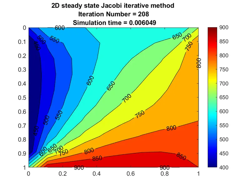
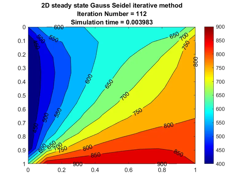
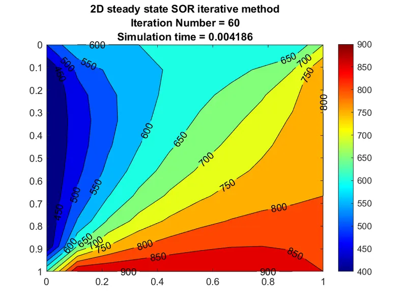
Unsteady/Transient state condition program:

As we know, Heat transfer is the transfer of thermal energy from a body at a high temperature to another at a lower temperature. This transfer of energy may occur under steady or unsteady state conditions. Under steady state conditions the temperature within the system does not change with time. Conversely, under unsteady state conditions the temperature within the system does vary with time.

Unsteady state conditions are a precursor to steady state conditions. No system exists initially under steady state conditions. After some time must pass, heat transfer is initiated before the system reaches steady state. During that period of transition, the system is under unsteady state conditions.

Clearly, no system can remain under unsteady state conditions perpetually. The temperature of the system will eventually reach the temperature of heat source and once this happens the system will be at steady state. Even if the amount of heat being transferred into it the starts causing phase changes within the system rather than temperatures increases.

Unsteady state situations appear after an imposed change in temperature at a boundary as well as inside of an object, as a result of new source or sink of heat suddenly introduced within an object, causing temperatures near the source or sink to change in time.

`(delT)/(delt)=alpha((del^2T)/(delx^2)+(del^2T)/(dely^2))`

If we discretise the equations it becomes,

`(T_(i,j)^(n+1)-T_(i,j)^n)/(Deltat)=alpha((T_(i,j-1)-2*T_(i,j)+T_(i,j+1))/(Deltax^2)+(T_(i-1,j)-2*T_(i,j)+T_(i+1,j))/(Deltay^2))^k`

In this above equation superscript k=n+1 for implicit and k=n for explicit

For Implicit

Implicit Approach is used in numerical analysis for obtaining numerical approximations to the solution of time dependent ordinary or partial differential equations as in required in computer simulations of a physical process.

Implicit methods find the solution by solving an equation involving both the current state of the system and the later one.

`T_(i,j)^(n+1)=T_(i,j)^n+alpha*Deltat*((T_(i,j-1)-2*T_(i,j)+T_(i,j+1))/(Deltax^2)+(T_(i-1,j)-2*T_(i,j)+T_(i+1,j))/(Deltay^2))^(n+1)`

If we simplify it further,

`T_(i,j)^(n+1)=1/(1+2*k_1+2*k_2)*(T_(i,j)^n+k_1(T_(i,j-1)+T_(i,j+1))^(n+1)+k_2(T_(i-1,j)+T_(i+1,j))^(n+1))`

here, CFL no. along x, `k_1=alpha*(Deltat)/(Deltax^2)` CFL no. along x, `k_1=alpha*(Deltat)/(Deltax^2)`

`alpha`is a diffusivity term, `alpha`=1.4 (considered arbitrarily)

For Explicit

Explicit methods calculate the state of a system at a later time by using data from the current state of system. In this method, each differential equation approach contains only one unknown and can be solved explicitly for this one unknown.

`T_(i,j)^(n+1)=T_(i,j)^n+alpha*Deltat*((T_(i,j-1)-2*T_(i,j)+T_(i,j+1))/(Deltax^2)+(T_(i-1,j)-2*T_(i,j)+T_(i+1,j))/(Deltay^2))^n`

If we simplify it further,

`T_(i,j)^(n+1)=T_(i,j)^n+k_1(T_(i,j-1)-2*T_(i.j)+T_(i,j+1))^n+k_2(T_(i-1,j)-2*T_(i,j)+T_(i+1,j))^n`

explicit diffusion problem, `CFL_(Total)<=0.5 i.e. CFL_x+CFL_y<=0.5`

if `CFL>0.5`...........solution becomes unstable

% Unsteady/Transient 2D heat conduction problem
% dT/dt=(d^2T/dx^2)+(d^2T/dy^2)
clear all 
close all
clc

% Inputs
nx=10; ny=10;
x=linspace(0,1,nx);
y=linspace(0,1,ny);
T=300*ones(nx,ny);

% Boundary condition
% T_top=600K ; T_bottom=900K ; T_left=400K ; T_right=800K
T(1,2:ny-1)=600;
T(nx,2:ny-1)=900;
T(2:nx-1,1)=400;
T(2:nx-1,ny)=800;
T(1,1)=500; T(1,ny)=700; T(nx,1)=650; T(nx,ny)=850;

% the domain is 1 metre in x & y direction
dx=x(2)-x(1);
dy=y(2)-y(1);

Tol=1e-4;
dt=0.001;
alpha=1.4;
T_old=T;
k1=alpha*(dt/dx^2);
k2=alpha*(dt/dy^2);
Term1=(1/(1+2*k1+2*k2));
Term2=k1*Term1;
Term3=k2*Term1;
iterative_solver=1;

% Implicit Method using jacobi
if iterative_solver == 1
    implicit_jac=implicit_2D_jacobi(Tol,nx,ny,T,T_old,Term1,Term2,Term3,x,y); 

% Implicit Method using gauss seidel
elseif iterative_solver == 2
  implicit_gs=implicit_2D_gauss_seidal(Tol,nx,ny,T,T_old,Term1,Term2,Term3,x,y);

% Implicit Method using SOR
elseif iterative_solver == 3
    implicit_sor=implicit_2D_sor(Tol,nx,ny,T,T_old,Term1,Term2,Term3,x,y); 

% Explicit Method
elseif iterative_solver == 4
    explicit_unsteady=explicit_2D_heat_conduction(Tol,nx,ny,k1,k2,T,T_old,x,y); 
end

• Function for implicit Jacobi iterative method

function T=implicit_2D_jacobi(Tol,nx,ny,T,T_old,Term1,Term2,Term3,x,y)
implicit_iter=1;
T_prev=T_old;
%Time loop
tic
for nt=1:1000
    error=9e9;
    % Convergence loop
    while(error>Tol)
        % Space loop
        for i=2:nx-1
            for j=2:ny-1
                H=(T_old(i,j-1)+T_old(i,j+1));
                V=(T_old(i-1,j)+T_old(i+1,j));
                T(i,j)=Term1*T_prev(i,j)+Term2*H+Term3*V;
            end
        end
        error=max(max(abs(T_old-T)));
        T_old=T;
        implicit_iter=implicit_iter+1;    
    end
    T_prev=T;
end
time1=toc;
figure(1)
contourf(x,y,T,'ShowText','on')
colorbar
colormap(jet)
set(gca,'ydir','reverse')
title_text=sprintf('2D Transient state Jacobi iterative method\nIteration Number = %d\nSimulation time = %f',implicit_iter,time1);
title(title_text)
end

• Function of Implicit Gauss-Seidel iterative method

function T=implicit_2D_gauss_seidal(Tol,nx,ny,T,T_old,Term1,Term2,Term3,x,y)
implicit_iter=1;
T_prev=T_old;
%Time loop
tic
for nt=1:1000
    error=9e9;
    % Convergence loop
    while(error>Tol)
        % Space loop
        for i=2:nx-1
            for j=2:ny-1             
                H=(T(i,j-1)+T(i,j+1));
                V=(T(i-1,j)+T(i+1,j));
                T(i,j)=Term1*T_prev(i,j)+Term2*H+Term3*V;
            end
        end
        error=max(max(abs(T_old-T)));
        T_old=T;
        implicit_iter=implicit_iter+1;      
    end
    T_prev=T;
end
time2=toc;
figure(1)
contourf(x,y,T,'ShowText','on')
colorbar
colormap(jet)
set(gca,'ydir','reverse')
title_text=sprintf('2D Transient state Gauss Seidel iterative method\nIteration Number = %d\nSimulation time = %f',implicit_iter,time2);
title(title_text)       
end

• Function for Implicit SOR iterative method

function T=implicit_2D_sor(Tol,nx,ny,T,T_old,Term1,Term2,Term3,x,y)
implicit_iter=1;
T_prev=T_old;
omega=1.1;
% Time loop
tic
for nt=1:1000
    error=9e9;
    % Convergence loop
    while(error>Tol)
        % Space loop
        for i=2:nx-1
            for j=2:ny-1
                H=(T(i,j-1)+T(i,j+1));
                V=(T(i-1,j)+T(i+1,j));
                T(i,j)=(1-omega)*T_old(i,j)+omega*(Term1*T_prev(i,j)+Term2*H+Term3*V);          
            end
        end
        error=max(max(abs(T_old-T)));
        T_old=T;
        implicit_iter=implicit_iter+1;        
    end
    T_prev=T;
end
time3=toc;
figure(1)
contourf(x,y,T,'ShowText','on')
colorbar
colormap(jet)
set(gca,'ydir','reverse')
title_text=sprintf('2D Transient state SOR iterative method\nIteration Number = %d\nSimulation time = %f',implicit_iter,time3);
title(title_text)
end

• Function for Explicit iteartive method

function T=explicit_2D_heat_conduction(Tol,nx,ny,k1,k2,T,T_old,x,y)
explicit_iter=1;
error=9e9;
% Time loop
tic
for nt=1:1000
    % Convergence loop
    while(error>Tol)
        % space loop
        for i=2:nx-1
            for j=2:ny-1
                Term1=T_old(i,j);
                Term2=k1*(T_old(i,j-1)-2*T_old(i,j)+T_old(i,j+1));
                Term3=k2*(T_old(i-1,j)-2*T_old(i,j)+T_old(i+1,j));
                T(i,j)=Term1+Term2+Term3;
            end
        end
        error=max(max(abs(T_old-T)));
        T_old=T;
        explicit_iter=explicit_iter+1;
    end
end
time4=toc;
figure(1)
contourf(x,y,T,'ShowText','on')
colorbar
colormap(jet)
set(gca,'ydir','reverse')
title_text=sprintf('2D Transient state Explicit iterative method\nIteration Number = %d\nSimulation time = %f', explicit_iter,time4);
title(title_text)
end

• Results:

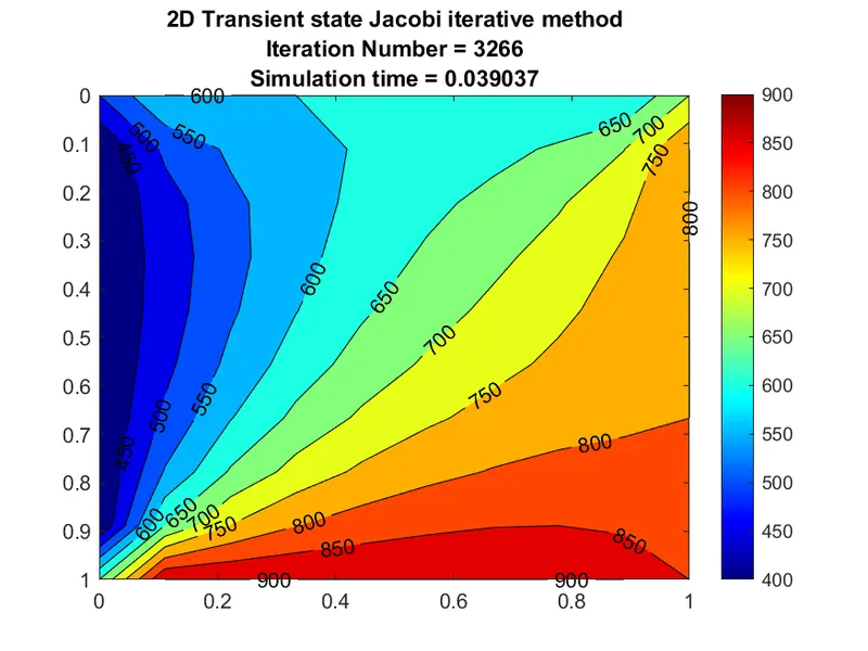
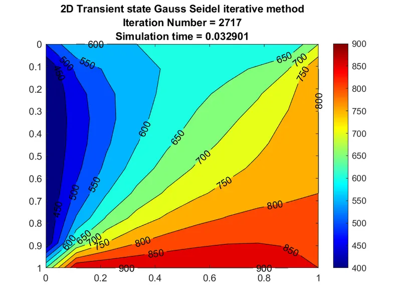
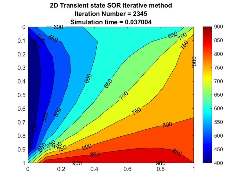
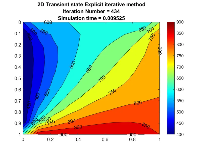
CONCLUSION:

Type of Scheme & Analysis	Various Method	No. of Iterations
IMPLICIT-Steady state Analysis	Jacobi	208
	Gauss-Siedel	112
	Successive Over Relaxation(SOR)	60
IMPLICIT-Transient state Analysis	Jacobi	3266
	Gauss-Siedel	2717
	Successive Over Relaxation(SOR)	2345
EXPLICIT Analysis		434

From the above outputs of various methods & compairing their No. of iterations, we can conclude that

• Jacobi > Gauss-Seidel > Successive over relaxation according to the no. of iterations computed for all methods & schemes.
• When compairing steady and transient state, due to compexity of equation of transient state take more no. of iterations to converge the solution and take more simulation time.
• For performing a simulation SOR method is more efficient to reach out solution quickly.