Week 3.5 - Deriving 4th order approximation of a 2nd order derivative using Taylor Table method

Aim: To derive and write a program in MATLAB for 4th order approximations of the second order derivative by follwing methods.

1. Central difference
2. Skewed right-sided difference
3. Skewed left-sided difference

Objective:

• To evaluate the second-order derivative of the analytical function `e^x*cos(x)` , Using above mentioned order approximations with the help of taylor table method.
• To plot and compare the values and errors of above derived methods.

Theory & Derivations:

During solving a CFD problem we may come across partial derivative equation which consists 2nd order derivative. Since due to complexity of the equation we may have to chose numerical approach and we try to make the error margin as low as possible. As the order of approximation get higher, we get higher accuracy.

According to the order of approximation, the number of nodes on the stencil changes. In order to derive the above differencing method we need to calculate the number of nodes on numerical stencil required to evaluate 4th order approximation of the second order derivative.

For Central Scheme:...........No. of nodes= p+q-1

No. of nodes= 2+4-1 = 5 node

For Skewd Scheme:............No. of nodes= p+q

No. of nodes= 2+4 = 6 node

where, p=order of derivative, q=order of approximation

1. Central differencing: For central scheme the nodes selected are symmetrical i.e the data is taken from the both sides of point of focus using Taylor's series.

The hypothesis of second order derivative is expressed as

`Deltax^2(del^2u)/(delx^2)=af(i-2)+bf(i-1)+cf(i)+df(i+1)+ef(i+2)`

Above hypothesis is expand with the help of taylor's series and rearrenging in the form of table using taylor table method.

`Deltax^2*(del^2u)/(delx^2)`	`f(i)`	`Deltaxf'(x)`	`Deltax^2f''(x)`	`Deltax^3f'''(x)`	`Deltax^4f''''(x)`
`af(i-2)`	a	-2a	4a/2	-8a/6	16a/24
`bf(i-1)`	b	-b	b/2	-b/6	b/24
`cf(i)`	c	0	0	0	0
`df(i+1)`	d	d	d/2	d/6	d/24
`ef(i+2)`	e	2e	4e/2	8e/6	16e/24
`Sigma(af(i-2)+bf(i-1)+cf(i)+df(i+1)+ef(i+2))`	0	0	1	0	0

the linear equation obtained from the above table and solved by matrix inversion method i.e. A*X=B

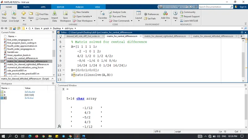
after solving the above matrix, we get the values of all the coefficients as:

a=-1/12, b=4/3, c=-5/2, d=4/3, e=-1/12

After putting values of coefficient(i.e. a,b,c,d,e) in above hypothesis equation, we will get central difference 4th order approximation of second order derivative.

`(del^2u)/(delx^2)=((-1/12)f(i-2)+(4/3)f(i-1)+(-5/2)f(i)+(4/3)f(i+1)+(-1/12)f(i+2))/(Deltax^2)`

2. Skewed right-sided differencing: When the data point of the left nodes are not available (at initial boundary conditions) then we have to rely on the available data set. such scheme are assymetric so we need to six nodes on numerical stencil required on the right hand side of point of focus in its differencing.

The hypothesis of second order derivative is expressed as

`Deltax^2(del^2u)/(delx^2)=af(i)+bf(i+1)+cf(i+2)+df(i+3)+ef(i+4)+gf(i+5)`

Above hypothesis expand with the help of taylor's series and rearranging in the form of table using taylor table method.

`Deltax^2(del^2u)/(delx^2)`	`f(i)`	`Deltaxf'(x)`	`Deltax^2f''(x)`	`Deltax^3f'''(x)`	`Deltax^4f''''(x)`	`Deltax^5f'''''(x)`
`af(i)`	a	0	0	0	0	0
`bf(i+1)`	b	b	b/2	b/6	b/24	b/120
`cf(i+2)`	c	2c	4c/2	8c/6	16c/24	32c/120
`df(i+3)`	d	3d	9d/2	27d/6	81d/24	243d/120
`ef(i+4)`	e	4e	16e/2	64e/6	256e/24	1024e/120
`gf(i+5)`	g	5g	25g/2	125g/6	625g/24	3125g/120
`Sigma(af(i)+bf(i+1)+cf(i+2)+df(i+3)+ef(i+4)+gf(i+5)`	0	0	1	0	0	0

The linear equation obtained by above table and solved by matrix inversion method i.e. A*X=B

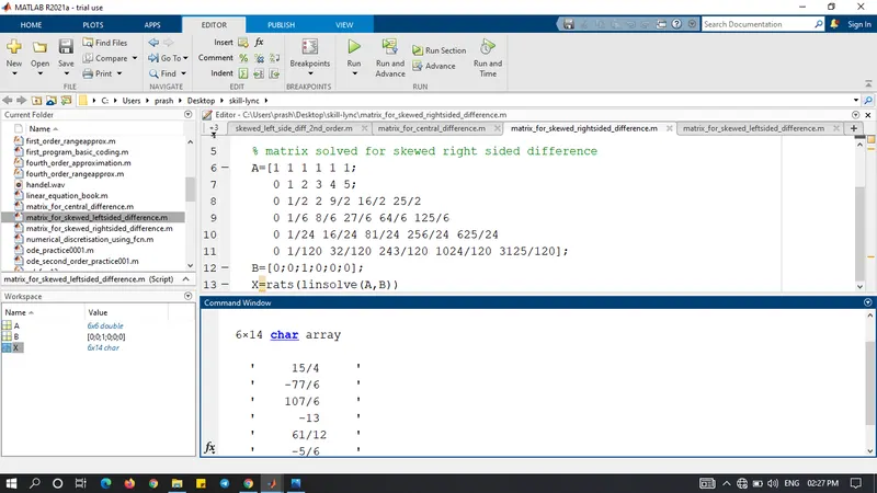
after solving above matrix, we get values of all the coefficient as:

a=15/4, b=-77/6, c=107/6, d=-13, e=61/12, g=-5/6

After putting values of coefficient(i.e. a,b,c,d,e,g) in above hypothesis equation, we will get skewed right sided differencing 4th order approximation of second order derivative.

`(del^2u)/(delx^2)=((15/4)f(i)+(-77/6)f(i+1)+(107/6)f(i+2)+(-13)f(i+3)+(61/12)f(i+4)+(-5/6)f(i+5))/(Deltax^2)`

3. Skewed left sided differencing: When the data point of the right nodes are not available(at boundary conditions) then we have to rely on the available data set. such scheme are assymetric so we need to six nodes on numerical stencil required on the left hand side of point of focus in its differencing.

The hypothesis of second order derivative is expressed as

`Deltax^2(del^2u)/(delx^2)=af(i-5)+bf(i-4)+cf(i-3)+df(i-2)+ef(i-1)+gf(i)`

Above hypothesis expand with yhe help of taylor's series and rearranging in the form of table using taylor table method

`Deltax^2(del^2u)/(delx^2)`	`f(i)`	`Deltaxf'(x)`	`Deltax^2f''(x)`	`Deltax^3f'''(x)`	`Deltax^4f''''(x)`	`Deltax^5f'''''(x)`
`af(i-5)`	a	-5a	25a/2	-125a/6	625a/24	-3125a/120
`bf(i-4)`	b	-4b	16b/2	-64b/6	256b/24	-1024b/120
`cf(i-3)`	c	-3c	9c/2	-27c/6	81c/24	-243c/120
`df(i-2)`	d	-2d	4d/2	-8d/6	16d/24	-32d/120
`ef(i-1)`	e	-e	e/2	-e/6	e/24	-e/120
`gf(i)`	g	0	0	0	0	0
`Sigma(af(i-5)+bf(i-4)+cf(i-3)+df(i-2)+ef(i-1)+gf(i)`	0	0	1	0	0	0

The linear equation obtained by above table and solved by matrix inversion method i.e. A*X=B

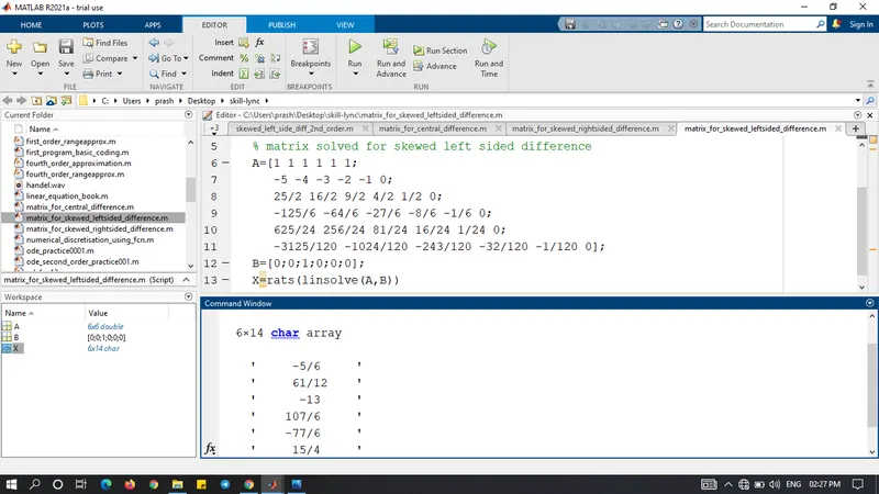
after solving above matrix we get values of all the coefficient as:

a=-5/6, b=61/12, c=-13, d=107/6, e=-77/6, g=15/4

After putting values of coefficient(i.e. a,b,c,d,e,g) in the above hypothesis equation, we will get skewed left sided differencing 4th order approximation of second order derivative.

`(del^2u)/(delx^2)=((-5/6)f(i-5)+(61/12)f(i-4)+(-13)f(i-3)+(107/6)f(i-2)+(-77/6)f(i-1)+(15/4)f(i))/(Deltax^2)`

MATLAB Code:

clear all
close all
clc

% value of x
x=pi/3;
% range of dx
dx=linspace(pi/4,pi/4000,40);
% Analytical function f(x)=exp(x)*cos(x)
% Analytical 2nd order derivative
analytical_derivative= -2*exp(x)*sin(x);

% Creating for loop
for i=1:length(dx)

% Central Difference
central_difference_error(i)=central_diff_2nd_order(x,dx(i),analytical_derivative);

% Skewed right sided difference
skewed_right_side_error(i)=skewed_right_side_diff_2nd_order(x,dx(i),analytical_derivative);

% Skewed left sided difference
skewed_left_side_error(i)=skewed_left_side_diff_2nd_order(x,dx(i),analytical_derivative);

end

% Plot graph
figure(1)
loglog(dx,central_difference_error,'r','Marker','o')
hold on
loglog(dx,skewed_right_side_error,'b','Marker','s')
hold on
loglog(dx,skewed_left_side_error,'g','Marker','d')
title('Consistency with different scheme')
xlabel('dx')
ylabel('Absolute error')
legend('Central difference of 4th order','Skewed right sided difference of 4th order','Skewed left sided difference of 4th order','location','NorthWest')
saveas(gcf,'Consistency with Central and skewed scheme','png')

• function for central difference

function error=central_diff_2nd_order(x,dx,analytical_derivative)

% Analytical function f(x)=exp(x)*cos(x)
% Numerical derivative
% f''(x)=((a*exp(x-2*dx)*cos(x-2*dx))+(b*exp(x-dx)*cos(x-dx))+(c*exp(x)*cos(x))+(d*exp(x+dx)*cos(x+dx))-(e*exp(x+2*dx)*cos(x+2*dx)))/(dx)^2;

% Central difference
central_difference=(((-1/12)*exp(x-2*dx)*cos(x-2*dx))+((4/3)*exp(x-dx)*cos(x-dx))+((-5/2)*exp(x)*cos(x))+((4/3)*exp(x+dx)*cos(x+dx))+((-1/12)*exp(x+2*dx)*cos(x+2*dx)))/(dx)^2;

error=abs(central_difference-analytical_derivative);

end

• function for skewed right sided difference

function error=skewed_right_side_diff_2nd_order(x,dx,analytical_derivative)

% Analytical function f(x)=exp(x)*cos(x)
% Numerical derivative
% f''(x)=((a*exp(x)*cos(x))+(b*exp(x+dx)*cos(x+dx))+(c*exp(x+2*dx)*cos(x+2*dx))+(d*exp(x+3*dx)*cos(x+3*dx))+(e*exp(x+4*dx)*cos(x+4*dx))+(g*exp(x+5*dx)*cos(x+5*dx)))/(dx)^2

% Skewed right side difference
skewed_right_side_difference=(((15/4)*exp(x)*cos(x))+((-77/6)*exp(x+dx)*cos(x+dx))+((107/6)*exp(x+2*dx)*cos(x+2*dx))+((-13)*exp(x+3*dx)*cos(x+3*dx))+((61/12)*exp(x+4*dx)*cos(x+4*dx))+((-5/6)*exp(x+5*dx)*cos(x+5*dx)))/(dx)^2;

error=abs(skewed_right_side_difference-analytical_derivative);

end

• function for left sided difference

function error=skewed_left_side_diff_2nd_order(x,dx,analytical_derivative)

% Analytical function f(x)=exp(x)*cos(x)
% Numerical derivative
% f''(x)=((a*exp(x-5*dx)*cos(x-5*dx))+(b*exp(x-4*dx)*cos(x-4*dx))+(c*exp(x-3*dx)*cos(x-3*dx))+(d*exp(x-2*dx)*cos(x-2*dx))+(e*exp(x-dx)*cos(x-dx))+(g*exp(x)*cos(x)))/(dx)^2;

% Skewed left side difference
skewed_left_side_difference=(((-5/6)*exp(x-5*dx)*cos(x-5*dx))+((61/12)*exp(x-4*dx)*cos(x-4*dx))+((-13)*exp(x-3*dx)*cos(x-3*dx))+((107/6)*exp(x-2*dx)*cos(x-2*dx))+((-77/6)*exp(x-dx)*cos(x-dx))+((15/4)*exp(x)*cos(x)))/(dx)^2;

error=abs(skewed_left_side_difference-analytical_derivative);

end

• Output

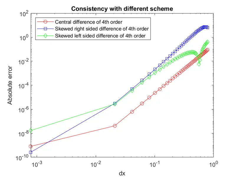
Conclusion:

• As we see in the graph between absolute error vs dx for central, skewed right-sided and skewed left-sided difference of 4th order error. we can easily notice that central difference approximation produce more accurate solution and produce lesser errors as compared to skewed right-sided and skewed left-sided schemes.

Describe why a skewed scheme is useful? What can a skewed scheme do that a CD scheme cannot do?

• Since we can see that the central differencing scheme gives us more accurate solutions or lesser errors as compared to the skewed difference scheme. But it is not always viable to use central differencing to evaluate solutions. Suppose , if we want to compute numerical approximations for a function at a boundary or corner node; we cannot use the central difference scheme at this particular situation because it requires data from both sides of node or boundary. So, in this situation skewed difference method plays an important role, as in the skewed scheme data from one side can be used to compute numerical approximation at a point.