Week 7 - Simulation of a 1D Super-sonic nozzle flow simulation using Macormack Method
main program
clear all
close all
clc

%SOLVING QUASI 1D SUPERSONIC NOZZLE FLOW EQUATIONS
%INPUT PARAMETERS
%No. of grid points
n = 31;

gamma = 1.4;
x = linspace(0,3,n);
dx = x(2) - x(1);

%No. of time step
nt = 1400;

%Courant Number
C = 0.5;


%FUNCTION FOR NON CONSERVATIVE FORM
tic;
[Mass_flow_rate_NC, Pressure_NC, Mach_number_NC, rho_NC, v_NC, T_NC, rho_throat_NC, v_throat_NC, T_throat_NC, Mass_flow_rate_throat_NC, Pressure_throat_NC, Mach_number_throat_NC] = Non_conservative_form(x, dx, n, gamma, nt, C);
Time_elapsed_NC = toc;
fprintf('Time Elasped for Non Conservative form: %0.4f', Time_elapsed_NC);
hold on

%PLOTTING
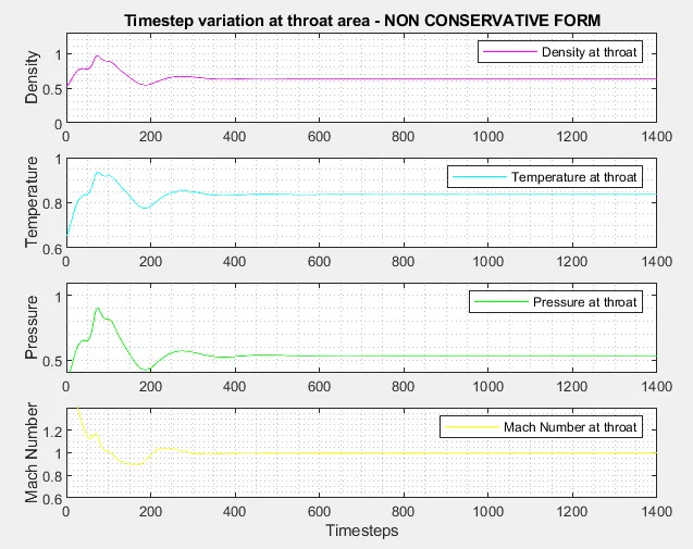
%Timestep variation of properties at throat area in Non Conservative form
figure(2)

%Density
subplot(4,1,1)
plot(linspace(1,nt,nt),rho_throat_NC,'color','m')
ylabel('Density')
legend({'Density at throat'});
axis([0 1400 0 1.3]);
grid minor;
title('Timestep variation at throat area - NON CONSERVATIVE FORM')

%Temperature
subplot(4,1,2)
plot(linspace(1,nt,nt),T_throat_NC,'color','c')
ylabel('Temperature')
legend({'Temperature at throat'});
axis([0 1400 0.6 1]);
grid minor;

%Pressure
subplot(4,1,3)
plot(linspace(1,nt,nt),Pressure_throat_NC,'color','g')
ylabel('Pressure')
legend({'Pressure at throat'});
axis([0 1400 0.4 1.1]);
grid minor

%Mach Number
subplot(4,1,4)
plot(linspace(1,nt,nt),Mach_number_throat_NC,'color','y')
xlabel('Timesteps')
ylabel('Mach Number')
legend({'Mach Number at throat'});
axis([0 1400 0.6 1.4]);
grid minor;


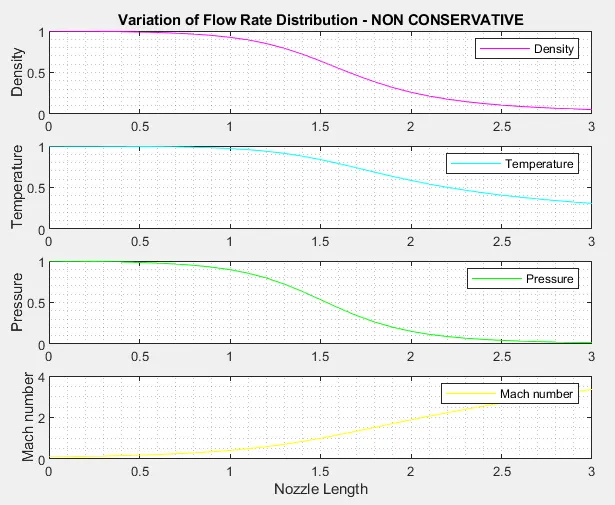
%Steady state simulation for primitve values for Non Conservative form
figure(3);
%Density

subplot(4,1,1);
plot(x,rho_NC,'color','m')
ylabel('Density')
legend({'Density'});
axis([0 3 0 1])
grid minor;
title('Variation of Flow Rate Distribution - NON CONSERVATIVE')

%Temperature
subplot(4,1,2);
plot(x,T_NC,'color','c')
ylabel('Temperature')
legend({'Temperature'});
axis([0 3 0 1])
grid minor;

%Pressure
subplot(4,1,3);
plot(x,Pressure_NC,'color','g')
ylabel('Pressure')
legend({'Pressure'});
axis([0 3 0 1])
grid minor;

%Mach number
subplot(4,1,4);
plot(x,Mach_number_NC,'color','y')
xlabel('Nozzle Length')
ylabel('Mach number')
legend({'Mach number'});
axis([0 3 0 4])
grid minor;


%FUNCTION FOR CONSERVATIVE FORM
tic;
[Mass_flow_rate_C, Pressure_C, Mach_number_C, rho_C, v_C, T_C, rho_throat_C, v_throat_C, T_throat_C, Mass_flow_rate_throat_C, Pressure_throat_C, Mach_number_throat_C] = Conservative_form(x, dx, n, gamma, nt, C);
Time_elasped_C = toc;
fprintf('Time Elasped for Conservative form: %0.4f', Time_elasped_C);

%PLOTTING
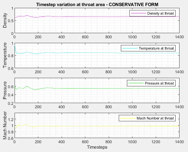
%Timestep variation of properties at throat area in Conservative form
figure(5)

%Density
subplot(4,1,1)
plot(rho_throat_C,'color','m')
ylabel('Density')
legend({'Density at throat'});
axis([0 1400 0 1]);
grid minor;
title('Timestep variation at throat area - CONSERVATIVE FORM')

%Temperature
subplot(4,1,2)
plot(T_throat_C,'color','c')
ylabel('Temperature')
legend({'Temperature at throat'});
axis([0 1400 0.6 1]);
grid minor;

%Pressure
subplot(4,1,3)
plot(Pressure_throat_C,'color','g')
ylabel('Pressure')
legend({'Pressure at throat'});
axis([0 1400 0.2 0.8]);
grid minor

%Mach Number
subplot(4,1,4)
plot(Mach_number_throat_C,'color','y')
xlabel('Timesteps')
ylabel('Mach Number')
legend({'Mach Number at throat'});
axis([0 1400 0.6 1.4]);
grid minor;


%Steady state simulation for primitve values for Non Conservative form
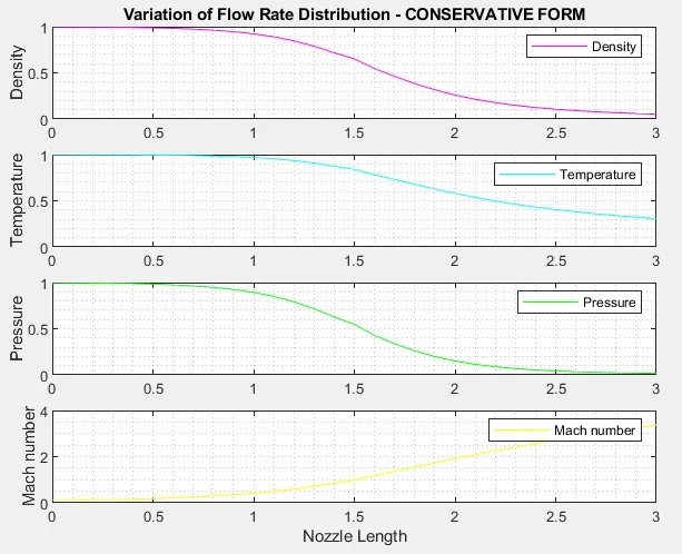
figure(6);

%Density
subplot(4,1,1);
plot(x,rho_C,'color','m')
ylabel('Density')
legend({'Density'});
axis([0 3 0 1])
grid minor;
title('Variation of Flow Rate Distribution - CONSERVATIVE FORM')

%Temperature
subplot(4,1,2);
plot(x,T_C,'color','c')
ylabel('Temperature')
legend({'Temperature'});
axis([0 3 0 1])
grid minor;

%Pressure
subplot(4,1,3);
plot(x,Pressure_C,'color','g')
ylabel('Pressure')
legend({'Pressure'});
axis([0 3 0 1])
grid minor;

%Mach number
subplot(4,1,4);
plot(x,Mach_number_C,'color','y')
xlabel('Nozzle Length')
ylabel('Mach number')
legend({'Mach number'});
axis([0 3 0 4])
grid minor;


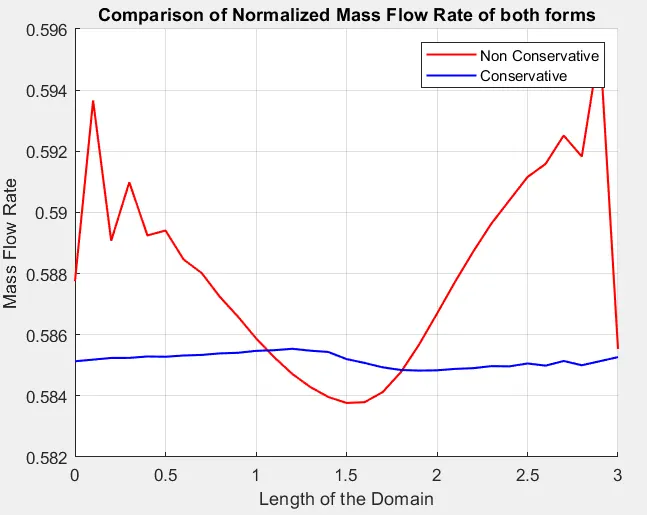
%COMPARISON PLOT of Normalized Mass Flow Rate of both forms
figure(7)
hold on
plot(x,Mass_flow_rate_NC,'r','linewidth',1.25)
hold on;
plot(x,Mass_flow_rate_C,'b','linewidth',1.25)
hold on;
grid on

legend('Non Conservative','Conservative');
xlabel('Length of the Domain')
ylabel('Mass Flow Rate')
title('Comparison of Normalized Mass Flow Rate of both forms')
Non conservative form
%Function for Non-Conservative form

function [Mass_flow_rate_NC, Pressure_NC, Mach_number_NC, rho_NC, v_NC, T_NC, rho_throat_NC, v_throat_NC, T_throat_NC, Mass_flow_rate_throat_NC, Pressure_throat_NC, Mach_number_throat_NC] = Non_conservative_form(x, dx, n, gamma, nt, C)

%Intial boundary conditions
rho_NC = 1 - 0.3146*x;
T_NC = 1 - 0.2341*x;
v_NC = (0.1 + 1.09*x).*T_NC.^0.5;

%Area & Throat profiles
a = 1 + 2.2*(x - 1.5).^2;
throat = find(a==1);


%Outer Time Loop
for k = 1:nt

    %Time-step control
    dt = min(C.*dx./(sqrt(T_NC) + v_NC));

    %Saving a copy of Old Values
    rho_old = rho_NC;
    T_old = T_NC;
    v_old = v_NC;


    %Predictor Method
    for j = 2:n-1

        %Simplifying the Equation's spatial terms
        dv_dx = (v_NC(j + 1) - v_NC(j))/dx;
        drho_dx = (rho_NC(j + 1) - rho_NC(j))/dx;
        dT_dx = (T_NC(j + 1) - T_NC(j))/dx;
        dlog_a_dx = (log(a(j + 1)) - log(a(j)))/dx;

        %Continuity Equation
        drho_dt_P(j) = -rho_NC(j)*dv_dx - rho_NC(j)*v_NC(j)*dlog_a_dx - v_NC(j)*drho_dx;

        %Momentum Equation
        dv_dt_P(j) = -v_NC(j)*dv_dx - (1/gamma)*(dT_dx + (T_NC(j)*drho_dx/rho_NC(j)));

        %Energy Equation
        dT_dt_P(j) = -v_NC(j)*dT_dx - (gamma - 1)*T_NC(j)*(dv_dx + v_NC(j)*dlog_a_dx);


        %Solution Update
        rho_NC(j) = rho_NC(j) + drho_dt_P(j)*dt;
        v_NC(j) = v_NC(j) + dv_dt_P(j)*dt;
        T_NC(j) = T_NC(j) + dT_dt_P(j)*dt;

    end


    %Corrector Method
    for j = 2:n-1

        %Simplifying the Equation's spatial terms
        dv_dx = (v_NC(j) - v_NC(j - 1))/dx;
        drho_dx = (rho_NC(j) - rho_NC(j - 1))/dx;
        dT_dx = (T_NC(j) - T_NC(j - 1))/dx;
        dlog_a_dx = (log(a(j)) - log(a(j - 1)))/dx;

        %Continuity Equation
        drho_dt_C(j) = - rho_NC(j)*dv_dx - rho_NC(j)*v_NC(j)*dlog_a_dx - v_NC(j)*drho_dx;

        %Momentum Equation
        dv_dt_C(j) = - v_NC(j)*dv_dx - (1/gamma)*(dT_dx + (T_NC(j)*drho_dx/rho_NC(j)));

        %Energy Equation
        dT_dt_C(j) = - v_NC(j)*dT_dx - (gamma - 1)*T_NC(j)*(dv_dx + v_NC(j)*dlog_a_dx);

    end

    %Compute Average Time derivative
    drho_dt = 0.5.*(drho_dt_P + drho_dt_C);
    dv_dt = 0.5.*(dv_dt_P + dv_dt_C);
    dT_dt = 0.5.*(dT_dt_P + dT_dt_C);

    %Final Solution Update
    for i = 2:n-1
        rho_NC(i) = rho_old(i) + drho_dt(i)*dt;
        v_NC(i) = v_old(i) + dv_dt(i)*dt;
        T_NC(i) = T_old(i) + dT_dt(i)*dt;

    end

    %Applying Boundary Conditions
    %At Inlet
    rho_NC(1) = 1;
    v_NC(1) = 2*v_NC(2) - v_NC(3);
    T_NC(1) = 1;

    %At Outlet
    rho_NC(n) = 2*rho_NC(n-1) - rho_NC(n - 2);
    v_NC(n) = 2*v_NC(n - 1) - v_NC(n - 2);
    T_NC(n) = 2*T_NC(n - 1) - T_NC(n - 2);


    %Defining Mass flow rate, Pressure and Mach number
    Mass_flow_rate_NC = rho_NC.*a.*v_NC;
    Pressure_NC = rho_NC.*T_NC;
    Mach_number_NC = (v_NC./sqrt(T_NC));

    %Calculating Variables at throat section
    rho_throat_NC(k) = rho_NC(throat);
    T_throat_NC(k) = T_NC(throat);
    v_throat_NC(k) = v_NC(throat);
    Mass_flow_rate_throat_NC(k) = Mass_flow_rate_NC(throat);
    Pressure_throat_NC(k) = Pressure_NC(throat);
    Mach_number_throat_NC(k) = Mach_number_NC(throat);


    %PLOTTING
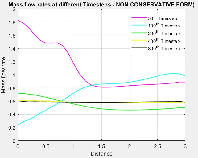
    %Comparison of non-dimensional Mass flow rates at different time steps
    figure(1);
    if k == 50
       plot(x, Mass_flow_rate_NC, 'm', 'linewidth', 1.25);
       hold on
    elseif k == 100
       plot(x, Mass_flow_rate_NC, 'c', 'linewidth', 1.25);
       hold on
    elseif k == 200
       plot(x, Mass_flow_rate_NC, 'g', 'linewidth', 1.25);
       hold on
    elseif k == 400
       plot(x, Mass_flow_rate_NC, 'y', 'linewidth', 1.25);
       hold on
    elseif k == 800
       plot(x, Mass_flow_rate_NC, 'k', 'linewidth', 1.25);
       hold on
    end

    %Labelling
    title('Mass flow rates at different Timesteps - NON CONSERVATIVE FORM)')
    xlabel('Distance')
    ylabel('Mass flow rate')
    legend({'50^t^h Timestep','100^t^h Timestep','200^t^h Timestep','400^t^h Timestep','800^t^h Timestep'})
    axis([0 3 0 2])
    grid on

end

end
Conservative form
%Function for Conservative form

function [Mass_flow_rate_C, Pressure_C, Mach_number_C,  rho_C, v_C, T_C, rho_throat_C, v_throat_C, T_throat_C, Mass_flow_rate_throat_C, Pressure_throat_C, Mach_number_throat_C] = Conservative_form(x, dx, n, gamma, nt, C)

%Determining Initial profile of Density and Temperature
for i = 1:n

    if (x(i) >= 0 && x(i) <= 0.5)
        rho_C(i) = 1;
        T_C(i) = 1;
    elseif (x(i) >= 0.5 && x(i) <= 1.5)
        rho_C(i) = 1 - 0.366*(x(i) - 0.5);
        T_C(i) = 1 - 0.167*(x(i) - 0.5);
    elseif (x(i) >= 1.5 && x(i) <= 3)
        rho_C(i) = 0.634 - 0.3879*(x(i) - 1.5);
        T_C(i) = 0.833 - 0.3507*(x(i) - 1.5);
    end

end

%Area & Throat profiles
a = 1 + 2.2*(x - 1.5).^2;
throat = find(a==1);

%Initial profile fot Velocity and Pressure
v_C = 0.59./(rho_C.*a);
Pressure_C = rho_C.*T_C;

%Calculate the Initial Solution Vectors(U)
U1 = rho_C.*a;
U2 = rho_C.*a.*v_C;
U3 = rho_C.*a.*(T_C./(gamma - 1)) + ((gamma/2).*v_C.^2);


%Outer Time Loop
for k =1:nt

    %Time-step control
    dt = min(C.*dx./(sqrt(T_C) + v_C));

    %Saving a copy of Old Values
    U1_old = U1;
    U2_old = U2;
    U3_old = U3;

    %Calculating the Flux vector(F)
    F1 = U2;
    F2 = ((U2.^2)./U1) + ((gamma - 1)/gamma)*(U3 - (gamma/2)*((U2.^2)./U1));
    F3 = ((gamma*U2.*U3)./U1) - (gamma*(gamma - 1)*((U2.^3)./(2*U1.^2)));


    %Predictor Method
    for j = 2:n-1

        %Calculating the Source term(J)
        J2(j) = (1/gamma)*rho_C(j)*T_C(j)*((a(j + 1) - a(j))/dx);


        %Continuity Equation
        dU1_dt_P(j) = -((F1(j + 1) - F1(j))/dx);

        %Momentum Equation
        dU2_dt_P(j) = -((F2(j + 1) - F2(j))/dx) + J2(j);

        %Energy Equation
        dU3_dt_P(j) = -((F3(j + 1) - F3(j))/dx);


        %Updating New values
        U1(j) = U1(j) + dU1_dt_P(j)*dt;
        U2(j) = U2(j) + dU2_dt_P(j)*dt;
        U3(j) = U3(j) + dU3_dt_P(j)*dt;

    end

    %Updating Flux vectors
    F1 = U2;
    F2 = ((U2.^2)./U1) + ((gamma - 1)/gamma)*(U3 - ((gamma*0.5*(U2.^2))./(U1)));
    F3 = ((gamma*U2.*U3)./U1) - ((gamma*0.5*(gamma - 1)*(U2.^3))./(U1.^2));


    %Corrector Method
    for j = 2:n-1

        %Updating the Source term(J)
        J2(j) = (1/gamma)*rho_C(j)*T_C(j)*((a(j) - a(j - 1))/dx);

        %Simplifying the Equation's spatial terms
        dU1_dt_C(j) = -((F1(j) - F1(j - 1))/dx);
        dU2_dt_C(j) = -((F2(j) - F2(j - 1))/dx) + J2(j);
        dU3_dt_C(j) = -((F3(j) - F3(j - 1))/dx);

    end

    %Compute Average Time derivative
    dU1_dt = 0.5*(dU1_dt_P + dU1_dt_C);
    dU2_dt = 0.5*(dU2_dt_P + dU2_dt_C);
    dU3_dt = 0.5*(dU3_dt_P + dU3_dt_C);

    %Final Solution Update
    for i = 2:n-1
        U1(i) = U1_old(i) + dU1_dt(i)*dt;
        U2(i) = U2_old(i) + dU2_dt(i)*dt;
        U3(i) = U3_old(i) + dU3_dt(i)*dt;

    end


    %Applying Boundary Conditions
    %At Inlet
    U1(1) = rho_C(1)*a(1);
    U2(1) = 2*U2(2) - U2(3);

    v_C(1) = U2(1)./U1(1);
    U3(1) = U1(1)*((T_C(1)/(gamma - 1)) + ((gamma/2)*(v_C(1)).^2));

    %At Outlet
    U1(n) = 2*U1(n - 1) - U1(n - 2);
    U2(n) = 2*U2(n - 1) - U2(n - 2);
    U3(n) = 2*U3(n - 1) - U3(n - 2);

    %Final Primitive value update
    rho_C = U1./a;
    v_C = U2./U1;
    T_C = (gamma - 1)*((U3./U1 - (gamma/2)*(v_C).^2));

    %Defining Mass flow rate, Pressure and Mach number
    Mass_flow_rate_C = rho_C.*a.*v_C;
    Pressure_C = rho_C.*T_C;
    Mach_number_C = (v_C./sqrt(T_C));

    %Calculating Variables at throat section
    rho_throat_C(k) = rho_C(throat);
    T_throat_C(k) = T_C(throat);
    v_throat_C(k) = v_C(throat);
    Mass_flow_rate_throat_C(k) = Mass_flow_rate_C(throat);
    Pressure_throat_C(k) = Pressure_C(throat);
    Mach_number_throat_C(k) = Mach_number_C(throat);

    %PLOTTING
    %Comparison of non-dimensional Mass flow rates at different time steps
    figure(4)
    if k == 50
       plot(x, Mass_flow_rate_C, 'm', 'linewidth', 1.25);
       hold on
    elseif k == 100
       plot(x, Mass_flow_rate_C, 'c', 'linewidth', 1.25);
       hold on
    elseif k == 200
       plot(x, Mass_flow_rate_C, 'g', 'linewidth', 1.25);
       hold on
    elseif k == 400
       plot(x, Mass_flow_rate_C, 'y', 'linewidth', 1.25);
       hold on
    elseif k == 800
       plot(x, Mass_flow_rate_C, 'k', 'linewidth', 1.25);
       hold on
    end


    %Labelling
    title('Mass flow rates at different Timesteps - CONSERVATIVE FORM')
    xlabel('Distance')
    ylabel('Mass flow rate')
    legend({'50^t^h Timestep','100^t^h Timestep','200^t^h Timestep','400^t^h Timestep','800^t^h Timestep'})
    axis([0 3 0.4 1])
    grid on

end

end
Time step variation at throat area
Non conservative form
conservative form
Variation of flow ratedistribution
mass flow rate at different timesteps
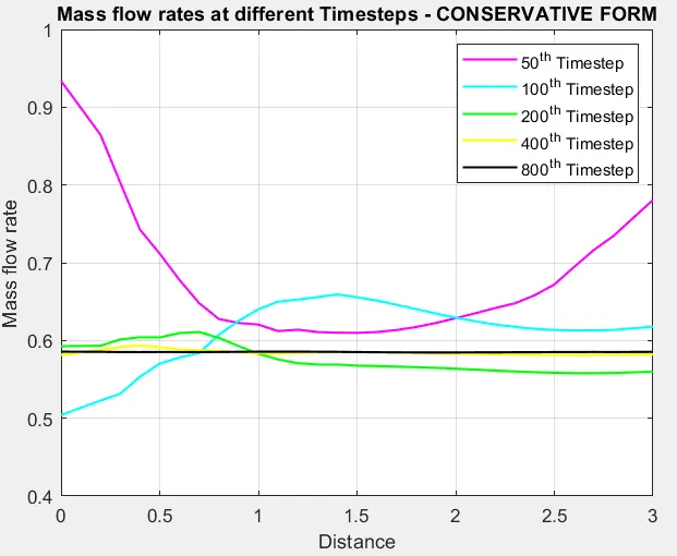
Comparision of normalized mass flow rate of both forms