Week 3.5 - Deriving 4th order approximation of a 2nd order derivative using Taylor Table method
1. Central differencing :- in central differencing we select the nodes in symmetrical.
by using Talor's method, we get
`(del^2f)/(delx^2) = af(i-2)+bf(i-1)+cf(i)+df(i+1)+ef(i+2)`
Taylor's tabel for cental differencing
f(x) dxf'(x) `dx^2f''(x)` `dx^3f'''(x)` `dx^4f''''(x)` `dx^5f'''''(x)`
af(i-1) a -2a 4a/2 -8a/6 16a/24 -32a/120
f(i-2) b -b b/2 -b/6 b/24 b/12
f(i) c 0 0 0 0 0
df(i-1) d d d/2 d/6 d/24 d/120
ef(i-2) e 2e 4e/2 8e/6 16e/24 32e/120
(af(i-2)+bf(i-1)+cf(i)
+df(i+1)+ef(i+2)) 0 0 1 0 0 ?
we convert the above tabel into matrix of type AX = B
[1 1 1 1 1 [ a [ 0
-2 -1 0 1 2 b 0
4/2 1/2 0 1/2 4/2 c 1
-8/6 -1/6 0 1/6 8/6 d 0
16/24 1/24 0 1/24 16/24 ] * e ] = 0 ]
on further solving we get the values
a=-0.0833
b=1.3333
c=-2.5000
d=1.3333
e=-0.0833
2. Skewed right side difference :the points of the left nodes are not avaliable
by using Talor's method, we get
`(del^2f)/(delx^2) = af(i)+bf(i+1)+cf(i+2)+df(i+3)+ef(i+4)+ff(i+5)`
Taylor's tabel for cental differencing
f(x) dxf'(x) `dx^2f''(x)` `dx^3f'''(x)` `dx^4f''''(x)` `dx^5f'''''(x)`
f(i) a 0 0 0 0 0
f(i+1) b b b/2 b/6 b/24 b/120
f(i+2) c 2c 4c/2 8c/6 16c/24 32c/120
df(i+3) d 3d 9d/2 27d/6 81d/24 243d/120
ef(i+4) e 4e 16e/2 64e/6 256e/24 1024e/120
ff(i+5) f 5f 25f/2 125f/6 625f/24 3125f/120
(af(i)+bf(i+1)+cf(i+2)
+df(i+3)+ef(i+4)+
ff(i+5)) 0 0 1 0 0 0
we convert the above tabel into matrix of type AX = B
[1 1 1 1 1 1 [ a [ 0
0 1 2 3 4 5 b 0
0 1/2 2 9/2 16/2 25/2 c 1
0 1/6 8/6 27/6 64/6 125/6 d 0
0 1/24 16/24 81/24 256/24 625/24 e 0
0 1/120 32/120 234/120 1024/120 3125/120 ] * f ] = 0 ]
on further solving we get the values
a=3.7500
b=-12.8333
c=17.8333
d=-13.0000
e=-5.0833
f=-0.8333
3. Skewed left side difference :the points of the right nodes are not avaliable
by using Talor's method, we get
`(del^2f)/(delx^2) = af(i-5)+bf(i-4)+cf(i-3)+df(i-2)+ef(i-1)+ff(i)`
Taylor's tabel for cental differencing
f(x) dxf'(x) `dx^2f''(x)` `dx^3f'''(x)` `dx^4f''''(x)` `dx^5f'''''(x)`
f(i) a -5a 25a/2 -125/6 625a/24 -3125a/120
f(i+1) b -4b 16b/2 -64/6 256/24 -1024b/120
f(i+2) c -3c 9c/2 -27c/6 81c/24 -234c/120
df(i+3) d -2d 4d/2 -8d/6 16d/24 -32d/120
ef(i+4) e -e e/2 -e/6 e/24 -e/120
ff(i+5) f 0 0 0 0 0
(af(i)+bf(i+1)+cf(i+2)
+df(i+3)+ef(i+4)+
ff(i+5)) 0 0 1 0 0 0
we convert the above tabel into matrix of type AX = B
[1 1 1 1 1 1 [ a [ 0
-5 -4 -3 -2 -1 0 b 0
25/2 16/2 9/2 2 1/2 1/2 c 1
-125/6 -64/6 -27/6 -8/6 -8/6 -1/6 d 0
625/24 256/24 81/24 16/24 16/24 1/24 e 0
-3125/120 -1024/120 -243/120 -32/120 -32/120 -1/120 ] * f ] = 0 ]
on further solving we get the values
a=-0.8333
b=5.0833
c=13.0000
d=17.8333
e=-12.8333
f=3.7500
main code :
clear all
close all
clc

%analytical function
x=pi/3;
dx=linspace(pi/10,pi/1000,100);
f=@(x)(exp(x)*cos(x));
g=@(x)(-2*exp(x)*sin(x));
d2f=g(x);
func=f(x);

%for central differencing
P=[1 1 1 1 1;-2 -1 0 1 2;4/2 1/2 0 1/2 4/2;-8/6 -1/6 0 1/6 8/6;16/24 1/24 0 1/24 16/24];
C=[0;0;1;0;0];
%P*a=C
cf1=P*C;


%for right skewed difference
Q=[1 1 1 1 1 1;0 1 2 3 4 5 ;0 1/2 2 9/2 16/2 25/2;0 1/6 8/6 27/6 64/6 125/6;0 1/24 16/24 81/24 256/24 625/24;0 1/120 32/120 243/120 1024/120 3125/120];
D=[0;0;1;0;0;0];
%Q*b=s
cf2=Q*D;


%for left skewed differencing
R=[1 1 1 1 1 1;-5 -4 -3 -2 -1 0;25/2 16/2 9/2 2 1/2 0;-125/6 -64/6 -27/6 -8/6 -1/6 0;625/24 256/24 81/24 16/24 1/24 0;-3125/120 -1024/120 -243/120 -32/120 -1/120 0];
E=[0;0;1;0;0;0];
%n*b=s
cf3=R*E;


%defining variable size
central_diff=zeros(1,100);
err_central=zeros(1,100);
right_sdiff=zeros(1,100);
err_right=zeros(1,100);
left_sdiff=zeros(1,100);
err_left=zeros(1,100);

for i=1:length(dx)

    %calculating value and error by central differencing
    central_diff(i)=(cf1(1)*f(x-2*dx(i))+cf1(2)*f(x-dx(i))+cf1(3)*f(x)+cf1(4)*f(x+dx(i))+cf1(5)*f(x+2*dx(i)))/(dx(i))^2;
    err_central(i)=abs(central_diff(i)-d2f);


    %calculating value and error by right skewed differencing
    right_sdiff(i)=(cf2(1)*f(x))+cf2(2)*f(x+dx(i))+cf2(3)*f(x+2*dx(i))+cf2(4)*f(x+3*dx(i))+cf2(5)*f(x+4*dx(i)+cf2(6)*f(x+5*dx(i)))/(dx(i))^2;
    err_right(i)=abs(right_sdiff(i)-d2f);


    %calculating value and error by left skewed differencing
    left_sdiff(i)=(cf3(1)*f(x-5*dx(i))+cf3(2)*f(x-4*dx(i))+cf3(3)*f(x-3*dx(i))+cf3(4)*f(x-2*dx(i))+cf3(5)*f(x-dx(i)+cf3(6)*f(x)))/(dx(i))^2;
    err_left(i)=abs(left_sdiff(i)-d2f);

end


%plotting errors in approximation of dervative

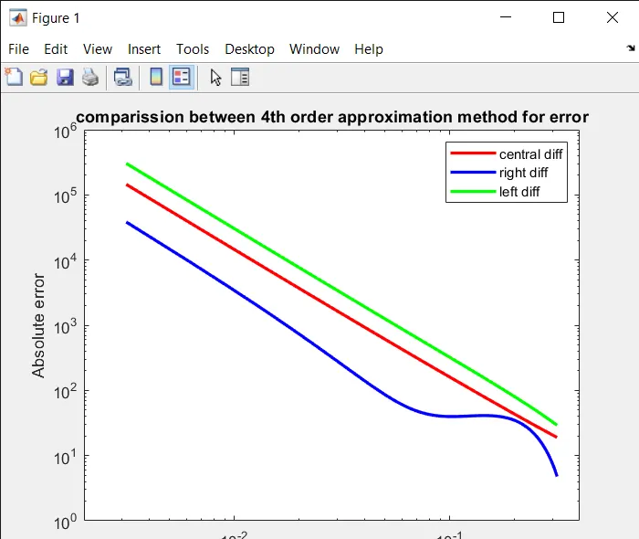
loglog(dx,err_central,'linewidth',2,'color','r');
hold on
xlim([0.002 0.4]);
loglog(dx,err_right,'linewidth',2,'color','b');
loglog(dx,err_left,'linewidth',2,'color','g');
legend('central diff','right diff','left diff')
xlabel('Grid sixe(dx)');
ylabel('Absolute error');
title('comparission between 4th order approximation method for error');