Week 7 - Simulation of a 1D Super-sonic nozzle flow simulation using Macormack Method
MacCormack's technique:
This technique will provide second order accuracy without involvement of second order derivative. According to this technique
`f^(n+1)=f^n+((delf)/((delt)avg))*(Deltat)`
This include a predictor step and a corrector step
Predictor step:
`(delf)/((delt)pred)=(f(i+1)-f(i))/(Deltat)`
Variables updated with using predictor derivative value
Corrector step
`(delf)/((delt)co)=(f(i)-f(i-1))/(Deltat)`
Final variables are updated using the average of predictor derivative and the corrector derivative.
Governing equation for quasi 1D supersonic nozzle flow
1. Non-conservative form
Continuity equation
`(delrho)/(delt)=rho*(delu)/(delx)-rho*u*(dellogA)/(delx)-u*(delp)/(delx)`
Momentum equation
`(delu)/(delt)=u*(delu)/(delx)-(1/gamma)*((delT)/(delx)+T/rho*(delrho)/(delx))`
Energy equation
`(delT)/(delt)=u*(delT)/(delx)-(gamma-1)*T*((delu)/(delx)+u*(dellogA)/(delx))`
These equations are solved using Maccormack's technique and proporties are evaluated
Inititial condition
Density `rho=1-(0.3146*x)`
Temperature `T=1-(0.2314*x)`
Velocity `u=(0.1+1.09*x)*T^0.5`
Area `A=1+(2.2*(x-1.5)^2)` where x is distance variable along nozzle axis
Boundary condition
At inlet `u(1)=2 *u(2)-u(3)`
At outlet
`u(n)=2 *u(n-1)-u(n-2)`
Temperature`T(n)=2 *T(n-1)-T(n-2)`
Density `rho(n)=2 *rho(n-1)-rho(n-2)`
The time step for this problem is obtained from CFL condition ( C=0.5)
`Deltat=min(C*(Deltax)/(sqrt(T)+V))`
2. Conservative form
For this we define certain terms
`U1=rho*A`,`U2=rho*A*u`,`U3=rho*((e)/(gamma-1)+(gamma)/2*u^2)`
`F1=U2`,`F2=rho*A*u^2*1/gamma*p*A`
`F3=rho*((e)/(gamma-1)+(gamma)/2*u^2)+1/gamma*p*A`
`J=1/gamma*p*(delA)/(delx)`
Continuity equation
`(delU1)/(delt)=-(delF1)/(delx)`
Momentum equation
`(delU2)/(delt)=-(delF2)/(delx)+J`
Energy equation
`(delU3)/(delt)=-(delF3)/(delx)`
Initial condition
`if 0<=x<=0.5`
`rho=1,T=1`
`if (x>0.5 )&&(x<=1.5)`
`rho=1-(0.366*(x-0.5)),T=1-(0.167*(x-0.5))`
else
`rho=0.634-(0.3879*(x-1.5)),T=0.833-(0.3507*(x-1.5))`
end
Boundary condition
Inlet
U1(1)=A(1)
U2(1)=2*U2(2)-U2(3)
`U3(1)=U1(1)*((T(1))/(gamma-1)+gamma/2*u^2)`
Outlet
`U1(n)=2 *U1(n-1)-U1(n-2)`
`U2(n)=2 *U2(n-1)-U2(n-2)`
`U3(n)=2 *U3(n-1)-U3(n-2)`
Main Programme
% Simulating of 1D super sonic nozzle flow using MACCORMACK'S Technique

close all;
clc;
clear;

% Grid point
n=31;
x=linspace(0,3,n);
dx=x(2)-x(1);
gamma=1.4;
% Total number of time step
nt=1400;
% Courant number
C=0.5;
% Area of nozzle
A=1+(2.2*(x-1.5).^2);
% Function for non-coservative form
 [V_nc,rho_nc,T_nc,m_nc,M_nc,P_nc,V_t_nc,rho_t_nc,T_t_nc,m_t_nc,M_t_nc,P_t_nc,non_conservative_run_time]=Non_conservative_form(x,dx,gamma,n,nt,C,A);

% Function for conservative form
[V_c,rho_c,T_c,m_c,M_c,P_c,V_t_c,rho_t_c,T_t_c,m_t_c,M_t_c,P_t_c,conservative_run_time]=Conservative_form(x,dx,gamma,n,nt,C,A);

% Exact value
m_e=linspace(0.579,0.579,n);
% Plotting
figure(3)
subplot(3,2,1)
plot(x,m_nc)
hold on
plot(x,m_c,'*')
plot(x,m_e,'--')
xlabel('Non-dimensional distance along nozzle axial direction')
ylabel('Mass flow rate')
title('Comparison of mass flow rate')
legend('Non-conservative form','Conservative form','Analytical solution')
grid on

subplot(3,2,2)
plot(x,M_nc)
hold on
plot(x,M_c,'*')
xlabel('Non-dimensional distance along nozzle axial direction')
ylabel('Mach number')
title('Comparison of mach number')
legend('Non-conservative form','Conservative form')

subplot(3,2,3)
plot(x,V_nc)
hold on
plot(x,V_c,'*')
xlabel('Non-dimensional distance along nozzle axial direction')
ylabel('Non-dimensational velocity')
title('Comparison of velocity')
legend('Non-conservative form','Conservative form')

subplot(3,2,4)
plot(x,rho_nc)
hold on
plot(x,rho_c,'*')
xlabel('Non-dimensional distance along nozzle axial direction')
ylabel('Non-dimensational density')
title('Comparison of density')
legend('Non-conservative form','Conservative form')

subplot(3,2,5)
plot(x,T_nc)
hold on
plot(x,T_c,'*')
xlabel('Non-dimensional distance along nozzle axial direction')
ylabel('Non-dimensational temperature')
title('Comparison of temperature')
legend('Non-conservative form','Conservative form')

subplot(3,2,6)
plot(x,P_nc)
hold on
plot(x,P_c,'*')
xlabel('Non-dimensional distance along nozzle axial direction')
ylabel('Pressure ratio')
title('Comparison of Pressure ratio')
legend('Non-conservative form','Conservative form')


figure(4)
subplot(4,1,1)
plot(1:nt,M_t_nc)
hold on
plot(1:nt,M_t_c)
xlabel('number of Time step')
ylabel('Mach number')
title('Comparison of mach number at throat')
legend('Non-conservative form','Conservative form')


subplot(4,1,2)
plot(1:nt,rho_t_nc)
hold on
plot(1:nt,rho_t_c)
xlabel('number of Time step')
ylabel('Density')
title('Comparison of density at throat')
legend('Non-conservative form','Conservative form')

subplot(4,1,3)
plot(1:nt,P_t_nc)
hold on
plot(1:nt,P_t_c)
xlabel('number of Time step')
ylabel('Pressure ratio')
title('Comparison of pressure ratio at throat')
legend('Non-conservative form','Conservative form')

subplot(4,1,4)
plot(1:nt,T_t_nc)
hold on
plot(1:nt,T_t_c)
xlabel('number of Time step')
ylabel('Temperature')
title('Comparison of temperature at throat')
legend('Non-conservative form','Conservative form')
Function code for Non-conservative form
function [V_nc,rho_nc,T_nc,m_nc,M_nc,P_nc,V_t_nc,rho_t_nc,T_t_nc,m_t_nc,M_t_nc,P_t_nc,non_conservative_run_time]=Non_conservative_form(x,dx,gamma,n,nt,C,A)
tic
drho_dt_p=zeros(n,1);
dV_dt_p=zeros(n,1);
dT_dt_p=zeros(n,1);
drho_dt_c=zeros(n,1);
dV_dt_c=zeros(n,1);
dT_dt_c=zeros(n,1);
V_t_nc=zeros(n,1);
rho_t_nc=zeros(n,1);
T_t_nc=zeros(n,1);
P_t_nc=zeros(n,1);
m_t_nc=zeros(n,1);
M_t_nc=zeros(n,1);
% Dimnsion less initial conditions
% Density rho_nc
rho_nc=1-.3146*x;
% Temperature T_nc
T_nc=1-.2314*x;
% Velocity V_nc
V_nc=(.1 + 1.09*x).*T_nc.^(0.5);
% Sonic speed
a=sqrt(T_nc);
% Time step
dt=min(C.*(dx./(a+V_nc)));

for k=1:nt
    rho_nc_old=rho_nc;
    V_nc_old=V_nc;
    T_nc_old=T_nc;

    % Predictor step
    for i=2:n-1
        drho_dx_p=(rho_nc(i+1)-rho_nc(i))/dx;
        dV_dx_p=(V_nc(i+1)-V_nc(i))/dx;
        dT_dx_p=(T_nc(i+1)-T_nc(i))/dx;
        dlogA_dx_p=(log(A(i+1))-log(A(i)))/dx;

        % Continuity Equation
        drho_dt_p(i)=-rho_nc(i)*dV_dx_p - rho_nc(i)*V_nc(i)*dlogA_dx_p - V_nc(i)*drho_dx_p;

        % Momentum Equation
        dV_dt_p(i)=-V_nc(i)*dV_dx_p-(1/gamma)*(dT_dx_p+(T_nc(i)/rho_nc(i))*drho_dx_p);

        % Energy Equation
        dT_dt_p(i)=-V_nc(i)*dT_dx_p-(gamma-1)*T_nc(i)*(dV_dx_p + (V_nc(i)*dlogA_dx_p));

        rho_nc(i)=rho_nc(i)+(drho_dt_p(i))*dt;
        V_nc(i)=V_nc(i)+(dV_dt_p(i))*dt;
        T_nc(i)=T_nc(i)+(dT_dt_p(i))*dt;
    end

    % Corrector step
    for i=2:n-1
        drho_dx_c=(rho_nc(i)-rho_nc(i-1))/dx;
        dV_dx_c=(V_nc(i)-V_nc(i-1))/dx;
        dT_dx_c=(T_nc(i)-T_nc(i-1))/dx;
        dlogA_dx_c=(log(A(i))-log(A(i-1)))/dx;

        % Continuity Equation
        drho_dt_c(i)=-rho_nc(i)*dV_dx_c - rho_nc(i)*V_nc(i)*dlogA_dx_c - V_nc(i)*drho_dx_c;

        % Momentum Equation
        dV_dt_c(i)=-V_nc(i)*dV_dx_c-(1/gamma)*(dT_dx_c+(T_nc(i)/rho_nc(i))*drho_dx_c);

        % Energy Equation
        dT_dt_c(i)=-V_nc(i)*dT_dx_c-(gamma-1)*T_nc(i)*(dV_dx_c + (V_nc(i)*dlogA_dx_c));
    end
    % Average derivative
    drho_dt_avg=0.5*(drho_dt_c+drho_dt_p);
    dV_dt_avg=0.5*(dV_dt_c+dV_dt_p);
    dT_dt_avg=0.5*(dT_dt_c+dT_dt_p);

    for i=2:n-1
        rho_nc(i)=rho_nc_old(i)+(drho_dt_avg(i))*dt;
        V_nc(i)=V_nc_old(i)+(dV_dt_avg(i))*dt;
        T_nc(i)=T_nc_old(i)+(dT_dt_avg(i))*dt;
    end

    % Boudary condition
    % Inlet
    V_nc(1)=2*V_nc(2)-V_nc(3);

    % Outlet
    V_nc(n)=2*V_nc(n-1)-V_nc(n-2);
    rho_nc(n)=2*rho_nc(n-1)-rho_nc(n-2);
    T_nc(n)=2*T_nc(n-1)-T_nc(n-2);

    % Mass flow rate
    m_nc=rho_nc.*A.*V_nc;

    % Pressure ratio
    P_nc=rho_nc.*T_nc;

    % Mach number M
    M_nc=V_nc./sqrt(T_nc);

    % Proporties at throat
    throat=(n+1)/2;
    rho_t_nc(k)=rho_nc(throat);
    V_t_nc(k)=V_nc(throat);
    T_t_nc(k)=T_nc(throat);
    P_t_nc(k)=P_nc(throat);
    m_t_nc(k)=m_nc(throat);
    M_t_nc(k)=M_nc(throat);

    % plotting of Mass flow rate
    figure(1)
    if k==50
        plot(x,m_nc,'r','lineWidth',1.5)
        hold on
    elseif k==100
        plot(x,m_nc,'b','lineWidth',1.5)
        hold on
    elseif k==150
        plot(x,m_nc,'y','lineWidth',1.5)
        hold on
    elseif k==200
        plot(x,m_nc,'g','lineWidth',1.5)
        hold on
    elseif k==700
        plot(x,m_nc,'*','lineWidth',1.5)
        hold on
    elseif k==1400
        plot(x,m_nc,'black','lineWidth',1.5)
        grid on
    end
end
xlabel('Non-dimensational distance in the nozzle axial direction')
ylabel('Non-dimensational mass flow rate through nozzle')
title({'Non-conservative form solution','Variation of mass flow rate along nozzle axial direction at different time'})
legend({'50 time steps','100 time steps','150 time steps','200 time steps','700 time steps','1400 time steps'})
non_conservative_run_time=toc;
end
Function code for Consrvative form
function [V_c,rho_c,T_c,m_c,M_c,P_c,V_t_c,rho_t_c,T_t_c,m_t_c,M_t_c,P_t_c,conservative_run_time]=Conservative_form(x,dx,gamma,n,nt,C,A)
tic
rho_c=zeros;
T_c=zeros;
J=zeros;
dU1_dt_p=zeros;
dU2_dt_p=zeros;
dU3_dt_p=zeros;
dU1_dt_c=zeros;
dU2_dt_c=zeros;
dU3_dt_c=zeros;
rho_t_c=zeros;
m_t_c=zeros;
P_t_c=zeros;
M_t_c=zeros;
V_t_c=zeros;
T_t_c=zeros;
% Initial canditions
% Density and Temperature
for i=1:n
    if (x(i)<=0.5)
        rho_c(i)=1;
        T_c(i)=1;
    elseif (x(i)>0.5) && (x(i)<=1.5)
        rho_c(i)=1-(0.366*(x(i)-0.5));
        T_c(i)=1-(0.167*(x(i)-0.5));
    else
        rho_c(i)=0.634-(0.3879*(x(i)-1.5));
        T_c(i)=0.833-(0.3507*(x(i)-1.5));
    end
end

% Velocity
V_c=(0.59)./(rho_c.*A);
% Sonic speed
a=sqrt(T_c);
% Time step
dt=min(C.*(dx./(a+V_c)));

% Set up for conservative form
U1=rho_c.*A;
U2=rho_c.*A.*V_c;
U3=rho_c.*A.*((T_c/(gamma-1))+(0.5*gamma.*V_c.*V_c));

for k=1:nt
    U1_old=U1;
    U2_old=U2;
    U3_old=U3;

    % Flux variables
    F1=U2;
    F2=((U2.^2)./U1)+((gamma-1)/gamma).*(U3-((gamma/2)*(U2.^2./U1)));
    F3=((gamma.*U2.*U3)./U1)-((gamma*(gamma-1))/2)*(U2.^3)./(U1.^2);

    % Predictor step

    for j=2:n-1
        dlogA_dx=(log(A(j+1))-log(A(j)))/dx;
        J(j)=dlogA_dx*((gamma-1)/gamma)*(U3(j)-(0.5*gamma*U2(j)^2)/(U1(j)));

        % Continuity Equation
        dF1_dx_p=(F1(j+1)-F1(j))/dx;
        dU1_dt_p(j)=-dF1_dx_p;

        % Momentum equation
        dF2_dx_p=(F2(j+1)-F2(j))/dx;
        dU2_dt_p(j)=-dF2_dx_p+J(j);

        % Energy Equation
        dF3_dx_p=(F3(j+1)-F3(j))/dx;
        dU3_dt_p(j)=-dF3_dx_p;

        U1(j)=(dU1_dt_p(j)*dt)+U1(j);
        U2(j)=(dU2_dt_p(j)*dt)+U2(j);
        U3(j)=(dU3_dt_p(j)*dt)+U3(j);
    end

    % Boundary condition
    % Input
    U1(1)=A(1);
    U2(1)=2*U2(2)-U2(3);
    U3(1)=U1(1)*((T_c(1)/(gamma-1)+((gamma/2)*V_c(1)^2)));

    % Output
    U1(n)=2*U1(n-1)-U1(n-2);
    U2(n)=2*U2(n-1)-U2(n-2);
    U3(n)=2*U3(n-1)-U3(n-2);

    % Updating
    F1=U2;
    F2=((U2.^2)./U1)+((gamma-1)/gamma).*(U3-((gamma/2)*(U2.^2./U1)));
    F3=((gamma.*U2.*U3)./U1)-((gamma*(gamma-1))/2)*(U2.^3)./(U1.^2);

    % Corrector step

    for j=2:n-1
        dlogA_dx=(log(A(j))-log(A(j-1)))/dx;
        J(j)=dlogA_dx*((gamma-1)/gamma)*(U3(j)-(0.5*gamma*U2(j)^2)/(U1(j)));

        % Continuity Equation
        dF1_dx_c=(F1(j)-F1(j-1))/dx;
        dU1_dt_c(j)=-dF1_dx_c;

        % Momentum equation
        dF2_dx_c=(F2(j)-F2(j-1))/dx;
        dU2_dt_c(j)=-dF2_dx_c+J(j);

        % Energy Equation
        dF3_dx_c=(F3(j)-F3(j-1))/dx;
        dU3_dt_c(j)=-dF3_dx_c;
    end

    % Average derivative
    dU1_dt_avg=0.5*(dU1_dt_c+dU1_dt_p);
    dU2_dt_avg=0.5*(dU2_dt_c+dU2_dt_p);
    dU3_dt_avg=0.5*(dU3_dt_c+dU3_dt_p);
    for j=2:n-1
        U1(j)=(dU1_dt_avg(j)*dt)+U1_old(j);
        U2(j)=(dU2_dt_avg(j)*dt)+U2_old(j);
        U3(j)=(dU3_dt_avg(j)*dt)+U3_old(j);
    end

    % Boundary condition
    % Input
    U1(1)=A(1);
    U2(1)=2*U2(2)-U2(3);
    U3(1)=U1(1)*((T_c(1)/(gamma-1)+((gamma/2)*V_c(1)^2)));

    % Output
    U1(n)=2*U1(n-1)-U1(n-2);
    U2(n)=2*U2(n-1)-U2(n-2);
    U3(n)=2*U3(n-1)-U3(n-2);

    % Primitive variables
    rho_c=U1./A;
    T_c=(gamma-1).*((U3./U1)-((gamma/2).*(U2./U1).^2));
    V_c=U2./U1;

    % Pressure ratio
    P_c=rho_c.*T_c;

    % Mach number
    M_c=V_c./(sqrt(T_c));

    % Mass flow rate
    m_c=rho_c.*V_c.*A;

    % Proporties at throat
    throat=(n+1)/2;
    rho_t_c(k)=rho_c(throat);
    V_t_c(k)=V_c(throat);
    T_t_c(k)=T_c(throat);
    P_t_c(k)=P_c(throat);
    m_t_c(k)=m_c(throat);
    M_t_c(k)=M_c(throat);

    % Plotting for mass flow rate
    figure(2)
    if k==50
        plot(x,m_c,'r','lineWidth',1.5)
        hold on
    elseif k==100
        plot(x,m_c,'b','lineWidth',1.5)
        hold on
    elseif k==150
        plot(x,m_c,'y','lineWidth',1.5)
        hold on
    elseif k==200
        plot(x,m_c,'g','lineWidth',1.5)
        hold on
    elseif k==700
        plot(x,m_c,'*','lineWidth',1.5)
        hold on
    elseif k==1400
        plot(x,m_c,'black','lineWidth',1.5)
        grid on
    end
end
xlabel('Non-dimensational distance in the nozzle axial direction')
ylabel('Non-dimensational mass flow rate through nozzle')
title({'Conservative form solution','Variation of mass flow rate along nozzle axial direction at different time'})
legend({'50 time steps','100 time steps','150 time steps','200 time steps','700 time steps','1400 time steps'})
conservative_run_time=toc;
end
Results
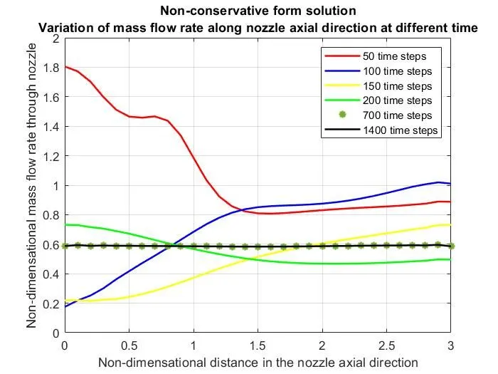
This figure shows the variation of mass flow rate at different time for non-conservative solution and we can observe the solution reached the steady state around 700 time steps.
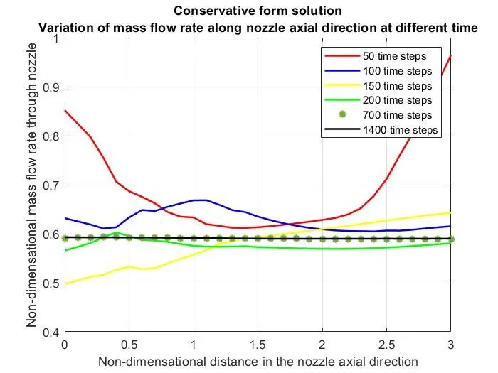
This figure shows the variation of mass flow rate with time for conservative form solution and we can observe that solution becomes steady at 700 time steps.
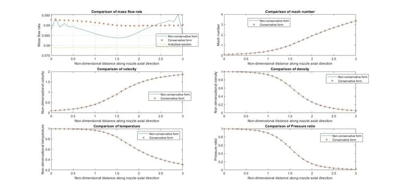
This figure shows the variation of primitive variables along nozzle axis for conservative and non-conservative solution. Except mass flow rate other proporties are same for both conservative and non-conservative solution. We can see that there is a fluctuation in mass flow rate in non-conservative solution and mass flow rate is stable in conservative solution.
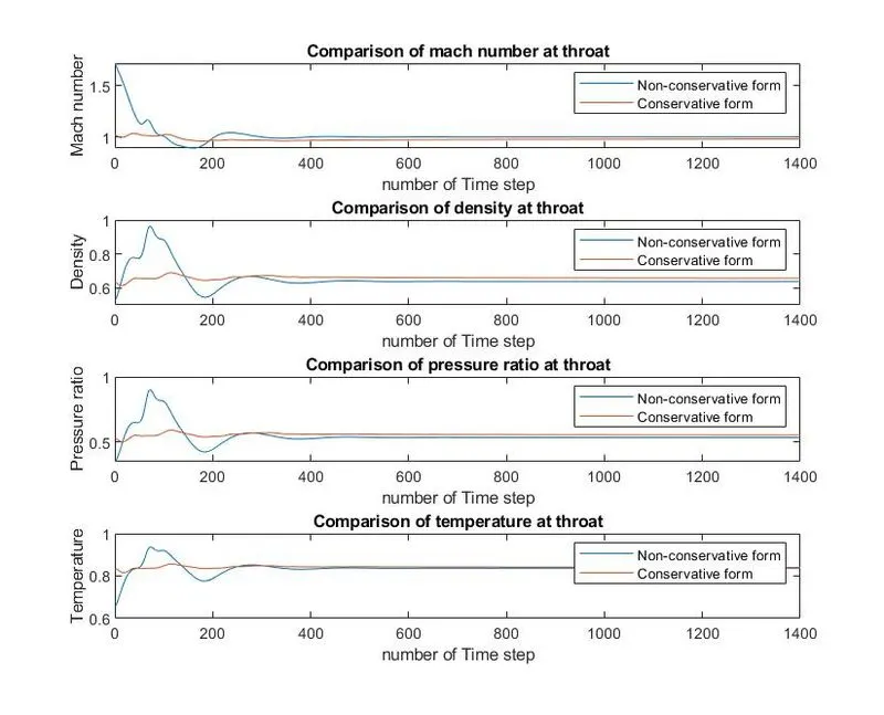
This figure shows the variation of different proporties at throat with time for both conservative and non-conservative solution. Initially solution is fluctuating , as time increases it becomes stable around 400 time steps.
Grid independence test
| Method | Nodes | rho_t | Mach number | T_t | P_t | Run time(s) |
| Non-conservative | 31 | 0.6387 | 0.9994 | 0.8365 | 0.5342 | 0.7155 |
| Non-conservative | 61 | 0.6377 | 0.9998 | 0.8354 | 0.5327 | 0.7011 |
| Conservative | 31 | 0.6571 | 0.9793 | 0.8407 | 0.5524 | 0.8334 |
| Conservative | 61 | 0.6403 | 0.9978 | 0.8357 | 0.5351 | 0.8398 |
| Analytical | - | 0.634 | 1 | 0.833 | 0.528 | - |
1.From the above table we can see that as grid point increases solutions become accurate.
2. With increase in accuracy computational time also increases.
Reference
1.JD Andersons CFD book