Week 4 - CHT Analysis on Exhaust port

Objective:

The objective of the problem is

1. Brief description of why and where a CHT analysis is used.
2. Maintain the y+ value according to the turbulence model and justify the results.
3. Calculate the wall/surface heat transfer coefficient on the internal solid surface & show the velocity & temperature contours in appropriate areas.
4. How would you verify if the HTC predictions from the simulations are right? On what factors does the accuracy of the prediction depend on?

Conjugate heat transfer:

Conjugate heat transfer corresponds with the combination of heat transfer in solids and heat transfer in fluids. In solids, conduction often dominates whereas in fluids, convection usually dominates. Conjugate heat transfer is observed in many situations, such as electronic cooling,turbine cooling and heat exchangers. After developement in computer performance to replace the emperical relation of heat transfer coefficient in numerical methods researchers started using conjugate heat transfer problem where there is conduction in solids and convection in fluids.

Introduction:

In this problem the hot fluid enters through inlet and flows through the exhaust port and the fluid is cooled by external convection from outer wall. So there is both conduction and convection. Generally we take external heat transfer coefficient by performing a simulation but in this case we assume it and perform the simulation.

Geometry setup:

Import the geometry in the spaceclaim and perform the following operation:

• prepare->volume extract-> select edge selection-> select all inside edges and click ok . Fluid volume will be extracted .
• Then in design change the name into solid domain and fluid domain.
• Then if you open the mesh and generate mesh then mesh will look like this

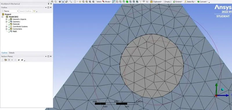
• As we can see there is a miss match between solid and fluid interface to fix this we will move both solid and volume to new component and delete empty components.
• Now click on share topology and share the geometry between the block is established. Now the geometry will look like

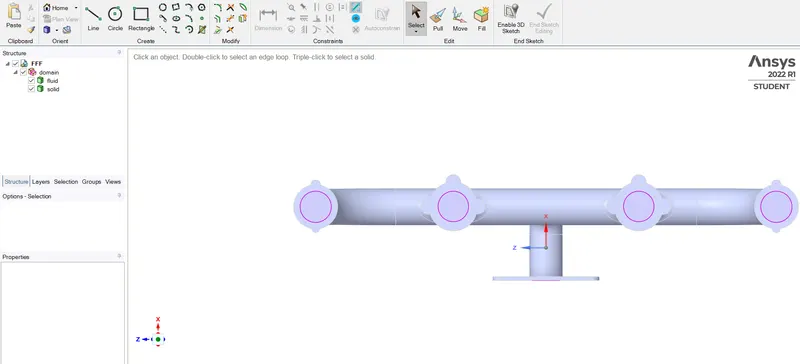
Meshing:

• First select names and give name for all the boundaries as inlet, outlet, outerwall_convection etc.
• Then give the inflation layers by calculating cell size from y plus.
• Select sizing for solid body and give element size 0.02 m.
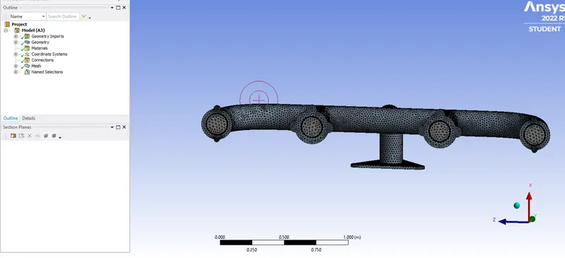
• Generate mesh and check quality it is greater than 0.2 .
• The mesh will look like

Problem setup:

• Select pressure based steady state solver and on energy mode.
• Among various turbulence models select k-wSST model.
• Solid is alluminium and fluid is air.
• Inlet is set at 5m/sec and 700K
• Outlet is atmospheric pressure.
• Outer wall convection is set at 20 w/M^2K heat transfer coefficient and support wall is set adiabatic.
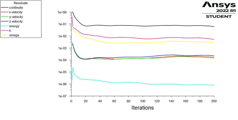
• Click on hybrid initialization and run for 200 iteration for converged solution.

Results:

The residual plot for this problem

The temperature contour plot at the outer wall

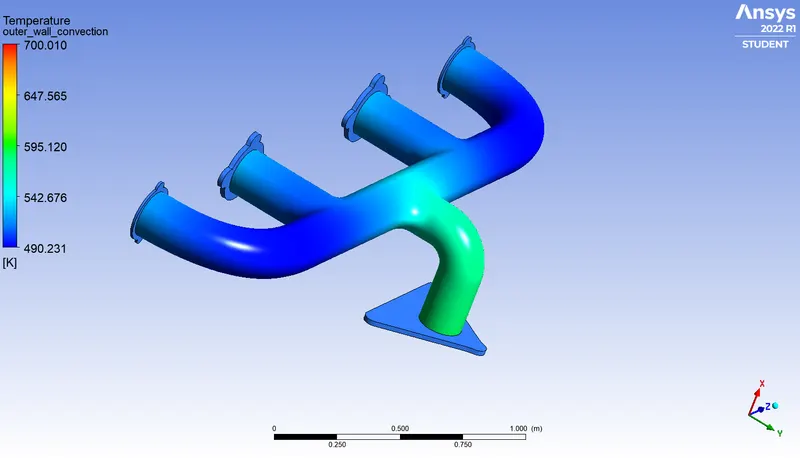
• As we can see from the plot the temperature of the wall at outlet is more compared to inlet because of convection.

We can see the stream line plot to locate maximum velocity

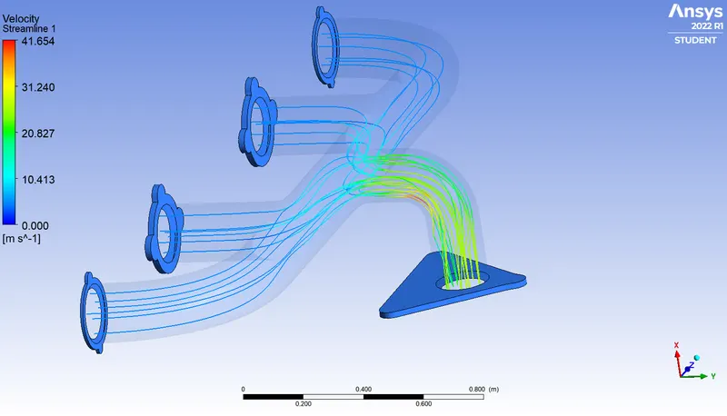
• As we can see from the streamline plot velocity is maximum at the outlet of the pipe compared to inlet this is because of mass conservation. As there are four inlet and one outlet and diameter of pipe is same and density is also constant , so velocity increases . We can see this in contour plot.

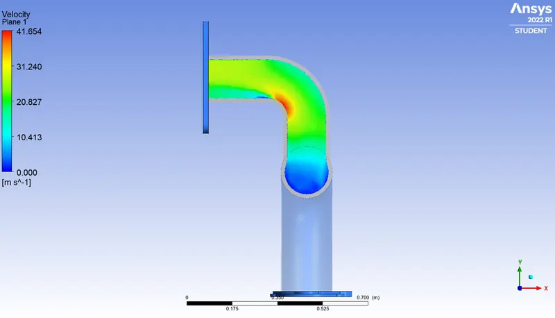
Velocity is increased from inlet to outlet.

If we see wall heat transfer coefficient plot

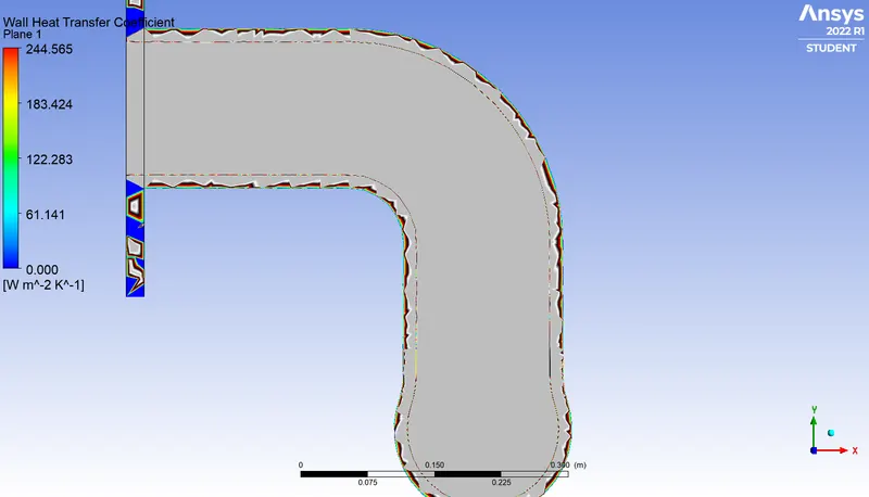
From the figure we can say that heat transfer coefficient is more at outlet.

We can verify the heat transfer coefficient by calculating from the following formula

`h=(0.023*Re^(4/5)*Pr^n*Kappa)/D`

where Re is reynould's number and Pr is Prandtle number

If we increase the Re number then the heat transfer coefficient increases.

yplus plot for the problem

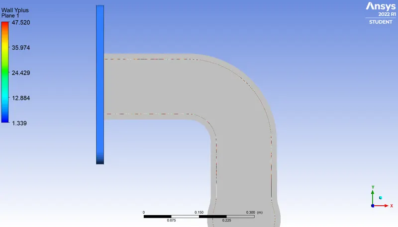
As we can see from the plot yplus is within 50 . If we use wall function then first grid should be at y plus 30 to 100. Without wall function y plus should be within 1 such cell size will be selected near wall.

Factors on the accuracy of the prediction depends

• Share topology must be selected between the domains.
• We need to enable share prep to fixing the interface problem.
• Appropriate turbulence model and selecting first grid near wall considering wall functions.
• Choosing outer wall heat transfer coefficient from simulation or from experimental results.
• Inflation layer near the wall.