Week 7 - Simulation of a 1D Super-sonic nozzle flow simulation using Macormack Method

Aim:

To simulate the isentropic flow through a quasi 1D subsonic-supersonic nozzle using MacCormack's technique in MATLAB.

Objectives:

- Derive both the conservation and non-conservation forms of the governing equations and sovle them using the MacCormack's technique.

- Required to determine the steady-state temperature distribution for the flow-field variables and investigate the difference between the two forms of governing equations by comparing their solutions.

Expected Results:

• Perform a grid independence test on the solution and expain all your findings.
• The code must be modular. You need to write separate functions to solve both forms.
• Discuss all the plots you are providing with observed inferences.

- Following plots are required to plot

1. Steady-state distribution of primitive variables inside the nozzle
2. Time-wise variation of the primitive variables
3. Variation of Mass flow rate distribution inside the nozzle at different time steps during the time-marching process
4. Comparison of Normalized mass flow rate distributions of both forms

Answer:

The schematic of subatomic - supersonic isentropic nozzle is shown below which has been taken from the Computational Fluid Dynamics book written by John D. Anderson.

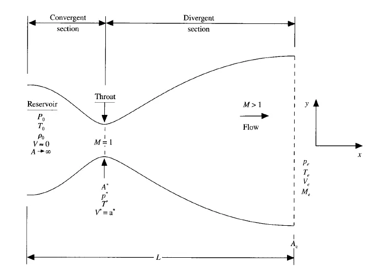
The above shown convergent-divergent nozzle receives the inlet from the reservoir where the pressure & temperature are `p_0` & `T_0`, respectively. The cross-sectional area of the reservoir is large, theoratically infinite, & that's why velocity will tends to zero. Thus, `p_0` & `T_0` are the stagnation values, or total pressure & total temperature, respectively. The flow expands isentropically to supersonic speeds at the nozzle exit, where the exit pressure, temperature, velocity & Mach number are denoted by `p_e`, `T_e`, `V_e` & `M_e`, respectively. The flwo is locally subsonic in the convergent section, sonic at the throat (minimum area) and supersonic at the divergent section. The sonic flow, M=1, at the throat means that the local velocity at this location is equal to the speed of sound.

Governing Equations:

Following non-dimensionless form of the variables are required to solve this problem:

`x^' = x/L` , `V^' = V/a_0`, `t^' = t/(L/a_0)`, `rho^' = rho/rho_0`, `T^' = T/T_0`, `p^' = p/p_0`, `A^' = A/A^**`

Following are the conservation & non-conservation form of the equations which will be solved in this problem.

1. Conservative Form

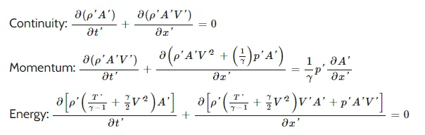
The conservative form of equations are made up of continuity, momentum & energy equations using non-dimensionless variables,

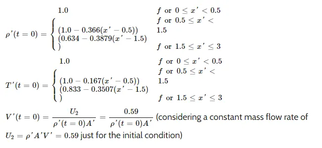
Initial conditions for this problem has been provided as follows,

2. Non-conservative Form

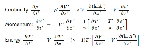
This form also has three mode of equations, which are continuity, energy & momentum. These equations also contain non-dimensionless varibles.

Initial conditions are also given for these equations to solve.

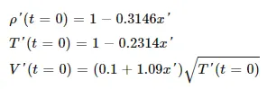
The above mentioned equations & the problem will be solved using MacCormic numerical scheme. This method is the most common method to solve the flow equations numerically. This method has four steps:

- Predictor Step

- Intermediate Step

- Corrector Step

- Final Solution Update

Main Code:

% Module - Introduction to CFD using MATLAB and OpenFOAM
% Week 7 challenge - Simulation of a 1D Super-sonic nozzle flow simulation
% using Macormack Method

close all
clear all
clc

% Input 
% Mesh grid
n =31;
x = linspace(0,3,n);
% difference between two points
dx = x(2) -x(1);
% Relaxation factor
gamma = 1.4;

% Courant number
cf = 0.5;

% no. of iterations
nt = 1400;

% initial profile area
a = 1+2.2*(x-1.5).^2;
% throat profile
thr = ((n-1)/2)+2;
% thr = find(a==1);


% executing function of non-consecutive & consecutive form of equations

% Non-conservative form
% measuring time
tic;
[v,rho,t,m,mach,p,v_t,rho_t,t_t,m_t,mach_t,p_t] = non_conservative(n,x,dx,cf,gamma,nt,a,thr);
% stopping time counter
time_nonconservative = toc;

% Conservative form
% measuring time
tic;
[v_c,rho_c,m_c_t,m_c,t_c,mach_c,p_c,v_c_t,rho_c_t,t_c_t,p_c_t,mach_c_t] = conservative_1(n,x,a,cf,dx,nt, gamma,thr);
% stopping time counter
time_conservative = toc;

% Plottting plots
% for mass flow rate
figure(3) 
plot(x,m)
hold on
plot(x,m_c,'o')
% plotting analytical solution
% mass flow rate = rho*a*v = 0.579
plot(x,linspace(0.579, 0.579,n));
grid on
xlabel('Nozzle Distance - Non dimensionalized')
ylabel('Mass flow rate - Non dimensionalized')
legend('Nonconservative Form', 'Conservative Form', 'Exact Analytical Solution')
title('Mass Flow Rate Comparision Between Conservative & Nonconservative Form')

% for Mach number
figure(4)
plot(x, mach)
hold on
plot(x,mach_c,'+')
grid on
xlabel('Nozzle Distance - Non dimensionalized')
ylabel('Mach Number')
legend('Nonconservative Form', 'Conservative Form')
title('Mach Number Across Nozzle in x')

% for pressure
figure(5)
plot(x,p)
hold on
plot(x,p_c,'*')
grid on
xlabel('Nozzle Distance - Non dimensionalized')
ylabel('Pressure')
legend('Nonconservative Form', 'Conservative Form')
title('Pressure Distribution Across Nozzle')

% for density
figure(6)
plot(x,rho)
hold on
plot(x,rho_c,'*')
grid on
xlabel('Nozzle Distance - Non dimensionalized')
ylabel('Density')
legend('Nonconservative Form', 'Conservative Form')
title('Density Distribution Across Nozzle')

% Nonconservative Form - Parameters Variables
figure(7)
subplot(4,1,1)
plot(x,mach)
ylabel('Mach Number')
title('Nonconservative Forms - Primitive Varialbes')
grid on
subplot(4,1,2)
plot(x, rho)
ylabel('Density')
grid on
subplot(4,1,3)
plot(x,p)
ylabel('Pressure')
grid on
subplot(4,1,4)
plot(x,t)
ylabel('Temperature')
grid on

% Conservative Form - Parameters Variables
figure(8)
subplot(4,1,1)
plot(x,mach_c)
ylabel('Mach Number')
title('Conservative Forms - Primitive Varialbes')
grid on
subplot(4,1,2)
plot(x, rho_c)
ylabel('Density')
grid on
subplot(4,1,3)
plot(x,p_c)
ylabel('Pressure')
grid on
subplot(4,1,4)
plot(x,t_c)
ylabel('Temperature')
grid on

% Primitive Variable at Nozzle Throat
figure(9)
subplot(4,1,1)
plot(1:nt,mach_t)
hold on
plot(1:nt,mach_c_t)
ylabel('Mach Number')
title('Varialbes at Nozzle Throat Cross Section For Both Forms')
legend('Nonconservative Form', 'Conservative Form')
grid on
subplot(4,1,2)
plot(1:nt, rho_t)
hold on
plot(1:nt, rho_c_t)
ylabel('Density')
legend('Nonconservative Form', 'Conservative Form')
grid on
subplot(4,1,3)
plot(1:nt,p_t)
hold on
plot(1:nt,p_c_t)
ylabel('Pressure')
legend('Nonconservative Form', 'Conservative Form')
grid on
subplot(4,1,4)
plot(1:nt,t_t)
hold on
plot(1:nt,t_c_t)
ylabel('Temperature')
legend('Nonconservative Form', 'Conservative Form')
grid on

Function for Nonconservative Form

function [v,rho,t,m,mach,p,v_t,rho_t,t_t,m_t,mach_t,p_t] = non_conservative(n,x,dx,cf,gamma,nt,a,thr)

% This function is associated with the Week 7 challenge - Simulation of a
% 1D Super-sonic nozzle flow simulation using Macormack Method.

% Function for Nonconservative form of equations.

% calculate initial profiles
rho = 1-0.3146*x; % density
t = 1-0.2314*x; % temperature
v = (0.1+1.09*x).*t.^0.5; % velocity

% time step size
dt = min(cf.*(dx./(sqrt(t)+v)));

% time loop
for k = 1:nt
    
    % storing values of previous iteration
    rho_old = rho;
    v_old = v;
    t_old = t;
    
    % predictor method
    for j = 2:n-1
        % drho_dt_p = -rho(j)*(v(j+1)-v(j))/dx - rho(j)*v(j)*(log(a(j+1)-log(a(j))))/dx - v(j)*(rho(j+1)-rho(j))/dx
        
        % Dividing main equation into smaller terms
        dvdx = (v(j+1)-v(j))/dx;
        drhodx = (rho(j+1)-rho(j))/dx;
        dtdx = (t(j+1)-t(j))/dx;
        dlogadx = (log(a(j+1))-log(a(j)))/dx;
        
        % Continuity Equation
        drhodt_p(j) = -rho(j)*dvdx -rho(j)*v(j)*dlogadx -v(j)*drhodx;
        
        % Momentum equation
        dvdt_p(j) = -v(j)*dvdx - (1/gamma)*(dtdx + (t(j)/rho(j))*drhodx);
        
        % energy equation
        dtdt_p(j) = -v(j)*dtdx - (gamma-1)*t(j)*(dvdx + v(j)*dlogadx);
        
        % Solution update
        rho(j) = rho(j) + drhodt_p(j)*dt;
        v(j) = v(j) + dvdt_p(j)*dt;
        t(j) = t(j) + dtdt_p(j)*dt;
    end
    
    % corrector method
    for j = 2:n-1
        % drho_dt_p = -rho(j)*(v(j+1)-v(j))/dx - rho(j)*v(j)*(log(a(j+1)-log(a(j))))/dx - v(j)*(rho(j+1)-rho(j))/dx
        
        % Dividing main equations into smaller terms
        dvdx = (v(j)-v(j-1))/dx;
        drhodx = (rho(j)-rho(j-1))/dx;
        dtdx = (t(j)-t(j-1))/dx;
        dlogadx = (log(a(j))-log(a(j-1)))/dx;
        
        % Continuity Equation
        drhodt_c(j) = -rho(j)*dvdx -rho(j)*v(j)*dlogadx -v(j)*drhodx;
        
        % Momentum equation
        dvdt_c(j) = -v(j)*dvdx - (1/gamma)*(dtdx + (t(j)/rho(j))*drhodx);
        
        % energy equation
        dtdt_c(j) = -v(j)*dtdx - (gamma-1)*t(j)*(dvdx + v(j)*dlogadx);
    end
    
    % Compute average time derivative
    drhodt = 0.5*(drhodt_p + drhodt_c);
    dvdt = 0.5*(dvdt_p + dvdt_c);
    dtdt = 0.5*(dtdt_p + dtdt_c);
    
    % Final solution update
    
    for i = 2:n-1
        rho(i) = rho_old(i) + drhodt(i)*dt;
        v(i) = v_old(i) + dvdt(i)*dt;
        t(i) = t_old(i) + dtdt(i)*dt;
    end
    
    % apply boundary condition
    % inlet
    v(1) = 2*v(2) - v(3);
    
    % outlet
    v(n) = 2*v(n-1) - v(n-2);
    rho(n) = 2*rho(n-1) - rho(n-2);
    t(n) = 2*t(n-1) - t(n-2);
    
    % properties
    m = rho.*a.*v; % mass flow rate
    p = rho.*t; % pressure
    mach = v./sqrt(t); % mach number
    
    % variables' values at nozzle throat
    rho_t(k) = rho(thr);
    v_t(k) = v(thr);
    t_t(k) = t(thr);
    p_t(k) = p(thr);
    mach_t(k) = mach(thr);
    m_t(k) = m(thr);
    
    % residuals
    rho_e = 0.634*ones(1,1400);
    t_e = 0.833*ones(1,1400);
    p_e = 0.528*ones(1,1400);
    mach_e = 1*ones(1,1400);
    
    % plots
    % Plotting mass flow rate during different time steps
    figure(1)
    if k == 200
        plot(x, m)
        hold on
    elseif k == 400
        plot(x,m)
        hold on
    elseif k ==600
        plot(x,m)
        hold on
    elseif k ==800
        plot(x,m)
        hold on        
    elseif k ==1000
        plot(x,m)
        hold on
    elseif k ==1400
        plot(x,m)
        hold on
    end
end

% Plot labels
xlabel('Diatance Through Nozzale in x Direction - Non dimensionalized')
ylabel('Mass Flow Rate - Non dimensionalized')
title('Mass Flow Rate - Different TimeStep - Nonconservative Form')
legend({'Time Step = 200', 'Time Step = 400', 'Time Step = 600', 'Time Step = 800', 'Time Step = 1000', 'Time Step = 1400'});

end

Function for Consertivaive Form

function [v_c,rho_c,m_c_t,m_c,mach_c, t_c,p_c,v_c_t,rho_c_t,t_c_t,p_c_t,mach_c_t] = conservative_1(n,x,a,cf,dx,nt, gamma,thr)

% This function is associated with the Week 7 challenge - Simulation of a
% 1D Super-sonic nozzle flow simulation using Macormack Method.

% Function for Conservative form of equations.

% loop to execute conservative form of equations according to their
% conditions
for i = 1:n
    if x(i)<= 0.5
        rho_initial(i) =1;
        t_initial(i) = 1;
    elseif (x(i)>=0.5) && (x(i)<=1.5)
        rho_initial(i)= 1-0.366*(x(i)-0.5);
        t_initial(i) = 1-0.167*(x(i)-0.5);
    elseif (x(i)>=1.5) && (x(i)<=3)
        rho_initial(i) = 0.634-0.3879*(x(i)-1.5);
        t_initial(i) = 0.833-0.3507*(x(i)-1.5);
    end
    v_initial(i) = 0.59./(rho_initial(i)*a(i));

end
    
% solution terms
u1 = rho_initial.*a;
u2 = rho_initial.*a.*v_initial;
u3 = u1.*((t_initial/(gamma-1))+(0.5*gamma*v_initial.^2));
p = rho_initial.*t_initial;

% time step size
dt = min(cf.*(dx./(sqrt(t_initial)+v_initial)));

% Primitive Variables
rho = rho_initial;
t = t_initial;
v = v_initial;

% main loop
for k = 1:nt
    
    % recording solution terms
    u1old = u1;
    u2old = u2;
    u3old = u3;
    
    % flux terms
    f1 = u2;
    
    term_1 = (((gamma-1)/gamma)*(u3-((gamma/2)*((u2.^2)./u1))));
    f2 = ((u2.^2)./u1)+term_1;
    f3 = ((gamma*u2.*u3)./u1)-((gamma/2)*(gamma-1)*(u2.^3))./(u1.^2);

    % predictor step
    for j = 2:n-1
        
        % Dividing main equation into smaller terms
        df1dx = (f1(j+1)-f1(j))/dx;
        df2dx = (f2(j+1)-f2(j))/dx;
        df3dx = (f3(j+1)-f3(j))/dx;
        dlogadx = (log(a(j+1))-log(a(j)))/dx;
        
        dadx = (a(j+1)-a(j))/dx;
        j2 = (1/gamma)*rho(j)*t(j)*dadx;
        
        % continuity equatjon
        du1dt_p(j) = -df1dx;
        
        % momentum equatjon
        du2dt_p(j) = -df2dx+j2;
        
        % energy equatjon
        du3dt_p(j) = -df3dx;
        
        % solution update
        u1(j) = u1(j)+du1dt_p(j)*dt;
        u2(j) = u2(j)+du2dt_p(j)*dt;
        u3(j) = u3(j)+du3dt_p(j)*dt;
    end
    
    % primitjve variables
    rho = u1./a;
    v = u2./u1;
    t = (gamma-1)*((u3./u1)-((gamma*v.^2)/2));
        
    % flux terms
    f1 = u2;
    
    term_1 = (((gamma-1)/gamma)*(u3-((gamma/2)*((u2.^2)./u1))));
    f2 = ((u2.^2)./u1)+term_1;
    f3 = ((gamma*u2.*u3)./u1)-((gamma/2)*(gamma-1)*(u2.^3))./(u1.^2);    
    
    % corrector step
    for q = 2:n-1
        df1dx = (f1(q)-f1(q-1))/dx;
        df2dx = (f2(q)-f2(q-1))/dx;
        df3dx = (f3(q)-f3(q-1))/dx;
        dlogadx = (log(a(q))-log(a(q-1)))/dx;
        
        dadx = (a(q)-a(q-1))/dx;
        j2 = (1/gamma)*rho(q)*t(q)*dadx;
        
        % continuity equatqon
        du1dt_c(q) = -df1dx;
        
        % momentum equatqon
        du2dt_c(q) = -df2dx+j2;
        
        % energy equatqon
        du3dt_c(q) = -df3dx;
    end
    
    % computing average time derivative
    du1dt = 0.5*(du1dt_p + du1dt_c);
    du2dt = 0.5*(du2dt_p + du2dt_c);
    du3dt = 0.5*(du3dt_p + du3dt_c);

    % final solution update
    for r = 2:n-1
         u1(r) = u1old(r)+du1dt(r)*dt;
         u2(r) = u2old(r)+du2dt(r)*dt;
         u3(r) = u3old(r)+ du3dt(r)*dt;
    end
    
    % inlet
    v(1) = u2(1)/u1(1);
    u1(1) = rho(1)*a(1);
    u2(1) = 2*u2(2)-u2(3);
    u3(1) = u1(1)*((t(1)/(gamma-1))+(0.5*gamma*v(1)^2));
    
    % outlet
    u1(n) = 2*u1(n-1)-u1(n-2);
    u2(n)=2*u2(n-1)-u2(n-2);
    u3(n)=2*u3(n-1)-u3(n-2);
    
    % primitive variables
    rho_c = u1./a; % density
    v_c = u2./u1; % velocity
    t_c = (gamma-1)*((u3./u1)-((gamma/2)*v.^2)); % temperature
   
    p_c = rho_c.*t; % pressure
    mach_c = v_c./(t_c.^0.5); % mach number
    m_c = rho_c.*v_c.*a; % mass flow rate
    
    % at throat
    rho_c_t(k) = rho_c(thr);
    v_c_t(k) = v_c(thr);
    t_c_t(k) = t_c(thr);
    p_c_t(k) = p_c(thr);
    mach_c_t(k) = mach_c(thr);
    m_c_t(k) = m_c(thr);
    
    % residuals
    u1_residual(k) = du1dt(thr);
    u2_residual(k) = du2dt(thr);
    u3_residual(k) = du3dt(thr);
    
    % plots
    % Plotting mass flow rate during different time steps
    figure(2)
    if k == 200
        plot(x, m_c)
        hold on
    elseif k == 400
        plot(x,m_c)
        hold on
    elseif k ==600
        plot(x,m_c)
        hold on
    elseif k ==800
        plot(x,m_c)
        hold on        
    elseif k ==1000
        plot(x,m_c)
        hold on
    elseif k ==1400
        plot(x,m_c)
        hold on
    end
end
    
% Plot labels
xlabel('Diatance Through Nozzale in x Direction - Non dimensionalized')
ylabel('Mass Flow Rate - Non dimensionalized')
title('Mass Flow Rate - Different TimeStep - Conservative Form')
legend({'Time Step = 200', 'Time Step = 400', 'Time Step = 600', 'Time Step = 800', 'Time Step = 1000', 'Time Step = 1400'});    
   
end

Results:

- The MaCormack method used in this problem shows very promising output for both forms of equations. The values are mostly very close to the analytical solutions. Because of this accuracy, it is widely used in solving flow problems. Following images will explain this graphically.

Figure 1

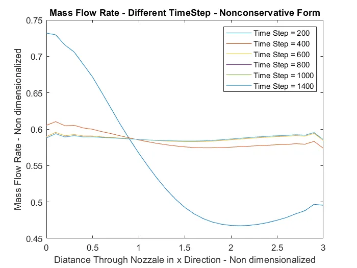
This image show the mass flow rate distribution across the nozzle during various time steps for non-conservative form. Except for 200 time step, the mass flow rate for any other time steps remain in the similar zone.

Figure 2

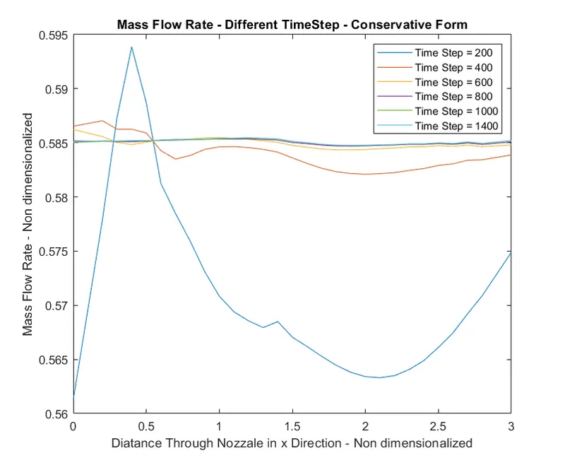
This result is for the conservative form. The results are similar to the non-conservative form. Only 200 timesteps line graph vary between 0.56 to 0.595 mass flow rate, while for all others, the values remained in the zone through out nozzle.

Figure 3

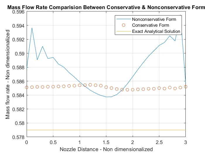
Figure 3 shows the comparison between conservative, non-conservative & analytical results. The conservative form has shown the similar graph across the nozzle with some difference in the value with analytical graph. The analytical solution is plotted at around 0.579 while the conservative form is plotted at 0.585. But the non-conservative form results are fluctuating throughout the nozzle.

Figure 4

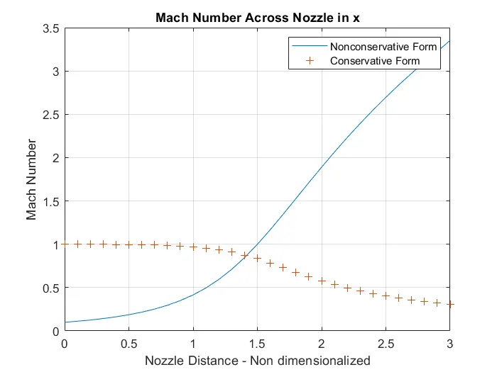
Figure 4 shows the comparision between Mach numbers of both forms across the length of nozzle. The mach number of non-conservative form is increasing steadily, especially after nozzle throat area, but the values for conservative form has been declining after the nozzle throat cross section.

Figure 5

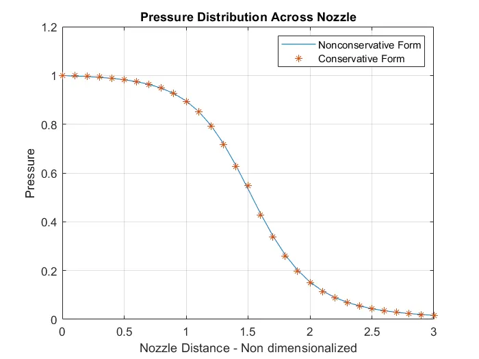
The pressure distribution for both forms have similar values across the nozzle length.

Figure 6

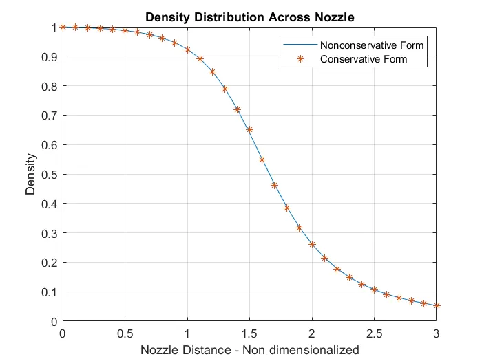
Similar way, the density distribution for both forms have also similar values across the nozzle length.

Figure 7

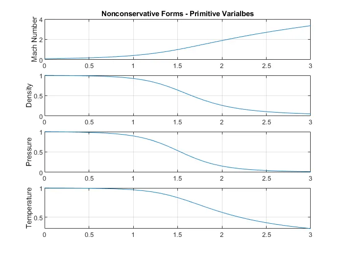
Figure 8

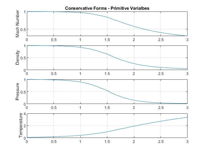
Figure 7 & 8, shows the variation in the variables across the length of nozzle for both forms. In Figure 7, the values are displayes for the non-conservative form while in figure 8, it is for conservative form.

The desnity & pressure has shown similar variation for both forms while for mach number plot & temperature plot has shown the reverse effect on the variables' values. For non-conservative form, the mach number is increasing steadily while for conservative form, it shows in decreasing manner. On the other hand, the temoerature plots have shown opposite effect on the values. The temperature values were increased while moving towards the end of nozzle for conservative form, but it displays decreasing for the other form.

Figure 9

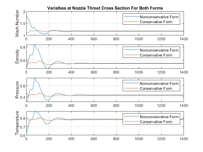
In the last image, the values of variables for both forms at nozzle throat cross section. Initially, the values were at different results, but mostly after 600 timesteps, both forms has been converge. In all four sublots, the nonconservative form has shown more variations than the conservative form.