Week 7 - Simulation of a 1D Super-sonic nozzle flow simulation using Macormack Method
Aim :
To simulate a 1D Super-sonic nozzle flow simulation using Macormack Method
Objective :
1. To use Matlab to solve the 1D isentropic flow through a convergent-divergent nozzle using Maccormack Technique.
2. To compare both conservative and non-conservative form of Navier stoke's equation to solve for the flow parameters.
Background:
Convergent-Divergent Nozzle
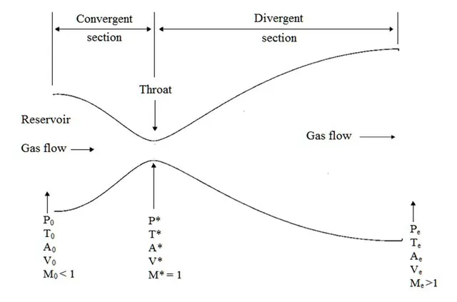
A nozzle is a device through which hot gases flow. Ramjets and rockets typically use a fixed convergent section followed by a fixed divergent section for the design of the nozzle. This nozzle configuration is called a convergent-divergent nozzle. In such a nozzle, the hot exhaust leaves the combustion chamber and converges down to the minimum area, or throat, of the nozzle.
The flow in the throat is sonic which means the Mach Number is equal to one in the throat.
Downstream of the throat, the geometry diverges and the flow is isentropically expanded to a supersonic Mach number that depends on the area of the exit to the throat.
The expansion of a supersonic flow causes the static pressure and temperature to decrease from the throat to the exit, so the amount of the expansion also determines the exit pressure and temperature.
The exit velocity, pressure, and mass flow through the nozzle determines the amount of thrust produced by the nozzle.
Solution Technique
The Maccormack method is an explicit finite-difference technique which is second-order-accurate in both space and time.
It is a 2-step predictor-corrector sequence that uses forward difference technique in predictor step and baclward difference in the corrector step.
`ρ_(i,j)^(t+dt) = ρ_(i,j)^(t)+((dp)/dt)_(av) * dt`
Where,
`((dρ)/dt)_(av) = 0.5 *[((dρ)/dt)_(pred)+((dρ)/dt)_(cr)]`
Predictor Step :
Taylor series with forward differencing is used to solve for the flow variables at time t+dt.
`(ρ)^(t+dt) = ρ_(i,j)^t + ((dρ)/dt)_(i,j)^t*dt`
Corrector Step :
In the corrector step, we first obtain a predicted value of the time derivative into the right side ofthe continuity equation, replacing the spatial derivatives with rearward differences.
Governing Equations :
At a given section, where the cross-sectional area is A, the flow properties are uniform across that section.
Hence, although the area of the nozzle changes as a function of distance along the nozzle, x, and therefore in reality the flow field is two-dimensional, we make the assumption that the flow properties-vary only with x this is tantamount to assuming uniform flow properties across any given cross section. Such flow is defined as quasi-one-dimensional flow.
1) Conservative Form
Continuity Equation :
`(∂(ρ'A'))/(∂t')+ (∂(ρ'A'V'))/(∂x') =0`
Momentum Equation :
`(∂(ρ'A'V'))/(∂t')+(∂(ρ'A'V^2)+(1/γ)*p'A')/(∂x') =0`
Energy Equation :
`(∂[ρ'((T')/(γ-1)+(γ/2*V^2)A')])/(∂t')+ (∂[ρ'((T')/(γ-1)+(γ/2*V^2)V'A')+p'A'V'])/(∂x')=0`
These equations are simplified by substituting the flux vectors and source terms.
`U_1 = ρ'A'`
`U_2 = ρ'A'V'`
`U_3=ρ'[(T/(γ-1))+(γ/2*V^2)]A'`
`F_1=ρ'A'V' = U_2`
`F_2=ρ'A'V'^2 +1/γp'A'`
`F_3=ρ'((T')/(γ-1)+(γ/2V'^2))V'A'+p'A'V'`
`J_2=1/γp'(∂A')/(∂x')`
Once the above equations are substituted, the governing equations become,
`(∂U_1)/(∂t')=-(∂F_1)/(∂x')`
`(∂U_2)/(∂t')=-(∂F_2)/(∂x')+J_2`
`(∂U_3)/(∂t')=-(∂F_3)/(∂x')`
2) Non-Conservative Form
Continuity Equation :
`(∂(ρ'))/(∂t')= -ρ(∂V')/(∂x') -ρ'V'(∂ (lnA')/(∂x'))-V'(∂ρ')/(∂x')`
Momentum Equation :
`(∂(V'))/(∂t')= -V'(∂V')/(∂x')-1/γ[(∂T)/(∂x')+(T')/(ρ')(∂ρ')/(∂x')]`
Energy Equation :
`(∂(T'))/(∂t')= -V'(∂T')/(∂x')-(γ-1)T'[(∂V)/(∂x')+V'(∂(lnA'))/(∂x')]`
Initial Conditions
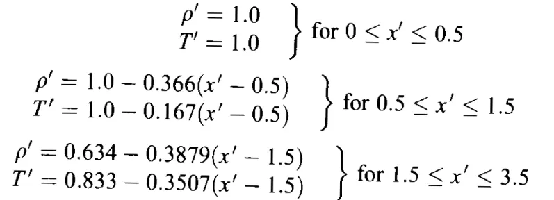
U2 is the local mass flow rate and is assumed to be
`U_2= ρ'A'V' =0.59`
Residual Plots
Mass Flow at various timesteps
Grid Dependency Test
Discussion of results
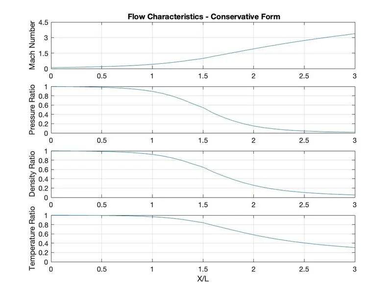
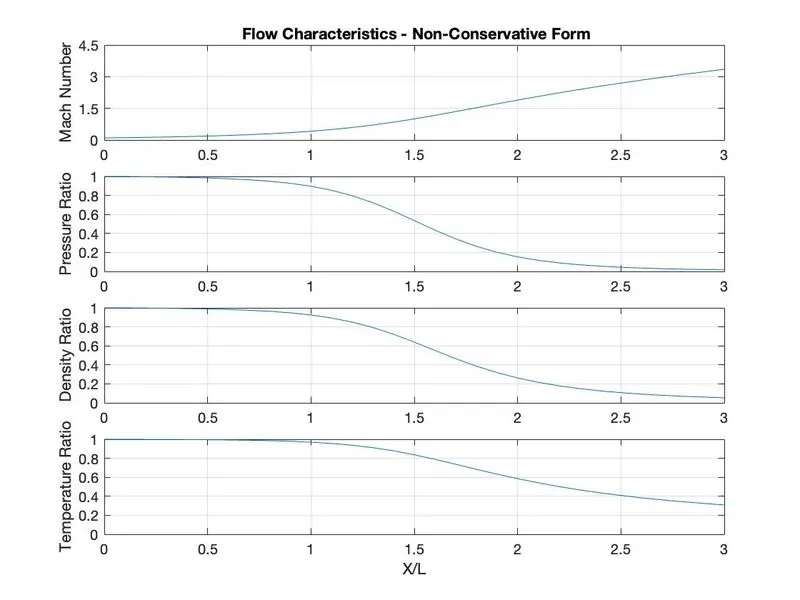
1) Flow Characteristics - From the flow characteristics of both conservarive and non-conservative form solutions, it can be ascertained that the mach number is 1 at the throat and it increases towards the diverging part of the nozzle.
It can also be noticed that all the non dimensional ratios increase along the length after the throat namely the Pressure, Density and Temperature ratio.
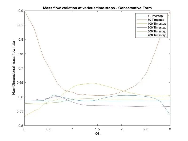
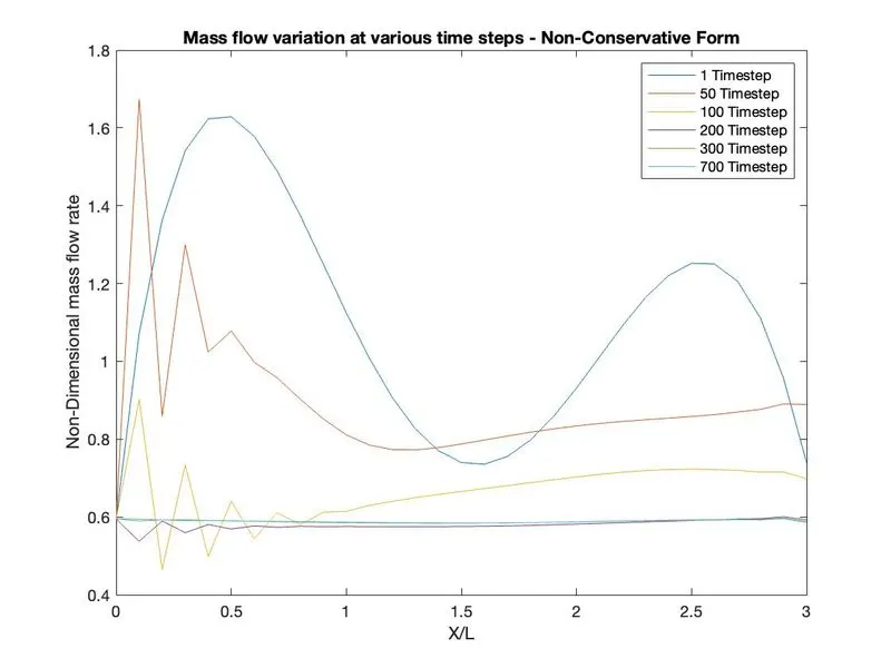
2) Massflow rate with time - For the Non-conservative form of the solution, at the initial timestep=1, the mass flow is observed to have fluctuations due to the initial assumption. However, beyond 200timestep, the solution was noticed to stabilize close to the analytical solution.
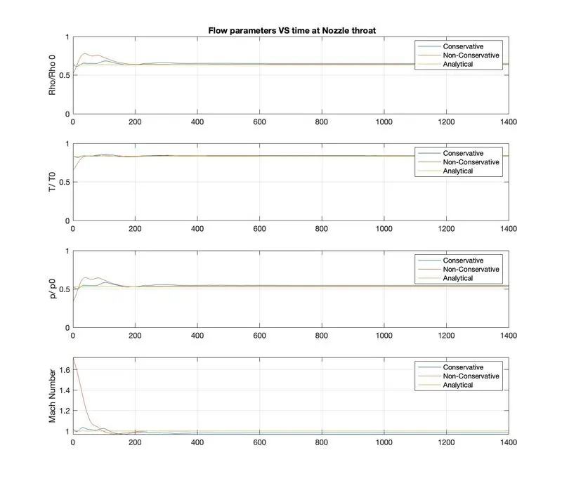
3) Non-Dimensional Parameters VS Time at throat - For both conservative and non-conservative solutions, the results were noticed to stabilize after 200seconds. It could also be noticed that the Non-Conservative solution is more close to the analytical solution.
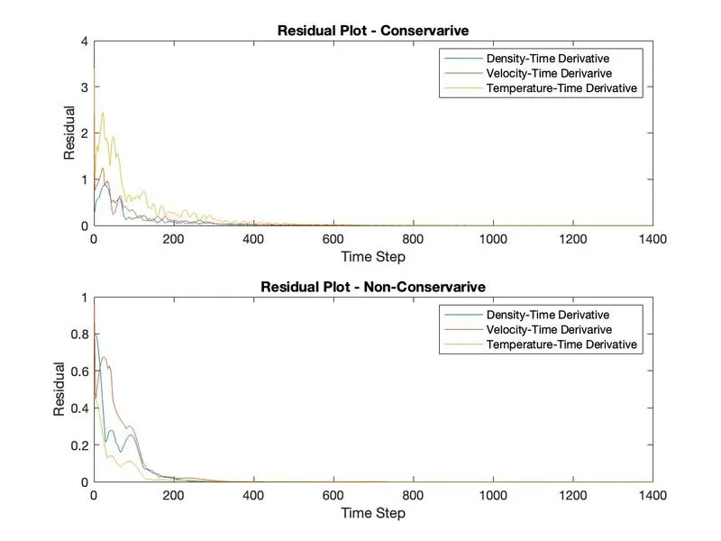
4) Residual Plots - Residuals are the absolute value of the time derivatives of the non-dimensional pressure, temperature and density /Source terms. The residuals oscilate and stabilize close to zero at timesteps greater than 500.
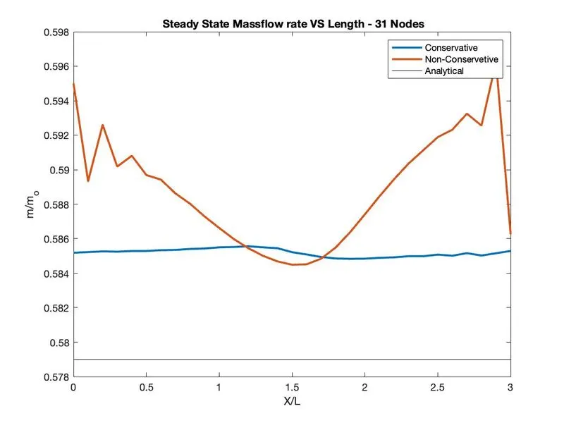
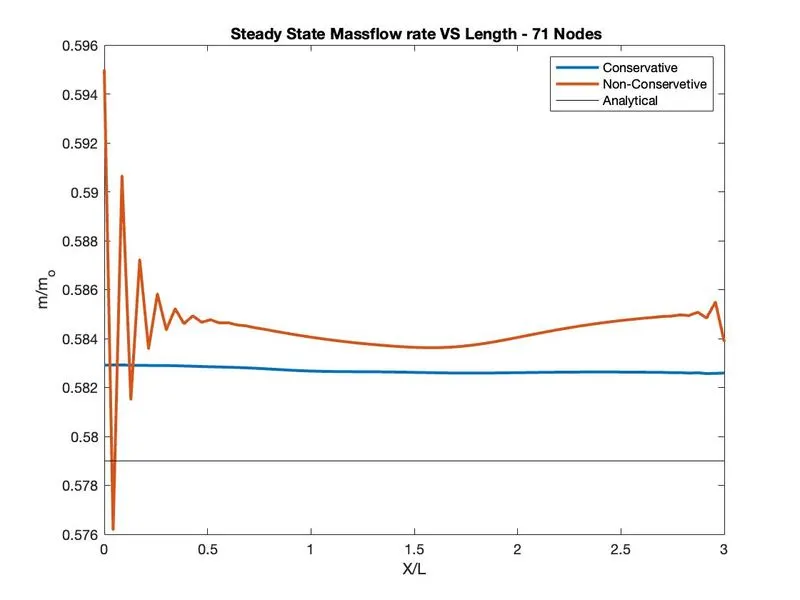
5) Grid Dependency - The steady state mass flow rate of the conservation form was noticed to be flatter and more accurate when compared with the non-conservative form.
Grid dependency was performed with nodes 31 and 71. The conservative form did not show much sensitivity to the number of nodes, however the Non-conservative form was noticed to be more stable with increased grid size.
Matlab Code
Main Code
clc
clear all
close all

L = 3; % Length of Nozzle
nx = [31]; % Number of Grid points
nt = 1400; % Number of timesteps
cfl = 0.5; % Courant Number

%% BC
x= linspace (0,L,nx)';
dx= x(2)-x(1);
A = 1+2.2*(x-1.5).^2;
gamma =1.4;

[rho1,V1,T1,p1,M1,m1,rho_throat1,V_throat1,p_throat1,T_throat1,M_throat1,res1]=Conservative_fn(x,dx,A,cfl,nt,gamma);
[rho2,V2,T2,p2,M2,m2,rho_throat2,V_throat2,p_throat2,T_throat2,M_throat2,res2]=NonConservative_fn(x,dx,A,cfl,nt,gamma);

%% Plotting Results - Figure1 Conservative

figure(1)
subplot(4,1,1)
plot(x,M1)
grid on;
ylim([0 4.5]);
yticks(0:1.5:4.5);
ylabel ('Mach Number');
title(' Flow Characteristics - Conservative Form');


subplot(4,1,2)
plot(x,p1)
grid on;
yticks(0:0.2:1);
ylabel ('Pressure Ratio');

subplot(4,1,3)
plot(x,rho1)
grid on;
yticks(0:0.2:1);
ylabel('Density Ratio');

subplot(4,1,4)
plot(x,T1)
grid on;
ylim([0 1]);
yticks(0:0.2:1);
ylabel('Temperature Ratio');
xlabel('X/L');

%% Figure2 Non-Conservative
figure(2)
subplot(4,1,1)
plot(x,M2)
grid on;
ylim([0 4.5]);
yticks(0:1.5:4.5);
ylabel ('Mach Number');
title(' Flow Characteristics - Non-Conservative Form');


subplot(4,1,2)
plot(x,p2)
grid on;
yticks(0:0.2:1);
ylabel ('Pressure Ratio');

subplot(4,1,3)
plot(x,rho2)
grid on;
yticks(0:0.2:1);
ylabel('Density Ratio');

subplot(4,1,4)
plot(x,T2)
grid on;
ylim([0 1]);
yticks(0:0.2:1);
ylabel('Temperature Ratio');
xlabel('X/L');
%% Throat flow parameters

rho_ana = 0.634*ones(1,1400);
T_ana = 0.833*ones(1,1400);
p_ana = 0.528*ones(1,1400);
M_ana = ones(1,1400);
m_ana =0.579*ones(length(x),1);


figure(3)
subplot(4,1,1)
plot(1:nt,rho_throat1)
hold on
plot(1:nt,rho_throat2)
hold on
plot(1:nt,rho_ana)
grid on;
ylim([0 1]);
ylabel('Rho/Rho 0');
title(' Flow parameters VS time at Nozzle throat');
legend('Conservative','Non-Conservative','Analytical');

subplot(4,1,2)
plot(1:nt,T_throat1)
hold on
plot(1:nt,T_throat2)
hold on
plot(1:nt,T_ana)
grid on;
ylim([0 1]);
ylabel('T/ T0');
legend('Conservative','Non-Conservative','Analytical');

subplot(4,1,3)
plot(1:nt,p_throat1)
hold on
plot(1:nt,p_throat2)
hold on
plot(1:nt,p_ana)
grid on;
ylim([0 1]);
ylabel('p/ p0');
legend('Conservative','Non-Conservative','Analytical');

subplot(4,1,4)
plot(1:nt,M_throat1)
hold on
plot(1:nt,M_throat2)
hold on
plot(1:nt,M_ana)
grid on;
ylabel('Mach Number');
legend('Conservative','Non-Conservative','Analytical');

%% Residual Plots

figure(4)
subplot(2,1,1)
plot(1:nt,res1);
xlabel('Time Step');
ylabel('Residual');
legend('Density-Time Derivative','Velocity-Time Derivarive','Temperature-Time Derivative');
title('Residual Plot - Conservarive');

subplot(2,1,2)
plot(1:nt,res2);
xlabel('Time Step');
ylabel('Residual');
legend('Density-Time Derivative','Velocity-Time Derivarive','Temperature-Time Derivative');
title('Residual Plot - Non-Conservarive');
%%
figure(5)
plot(x,m1(1,:))
hold on
plot(x,m1(50,:))
hold on
plot(x,m1(100,:))
hold on
plot(x,m1(200,:))
hold on
plot(x,m1(300,:))
hold on
plot(x,m1(700,:))
xlabel ('X/L')
ylabel('Non-Dimensional mass flow rate')
title('Mass flow variation at various time steps - Conservative Form')
legend('1 Timestep','50 Timestep','100 Timestep','200 Timestep','300 Timestep','700 Timestep');

figure(6)
plot(x,m2(1,:))
hold on
plot(x,m2(50,:))
hold on
plot(x,m2(100,:))
hold on
plot(x,m2(200,:))
hold on
plot(x,m2(300,:))
hold on
plot(x,m2(700,:))
xlabel ('X/L')
ylabel('Non-Dimensional mass flow rate')
title('Mass flow variation at various time steps - Non-Conservative Form')
legend('1 Timestep','50 Timestep','100 Timestep','200 Timestep','300 Timestep','700 Timestep');

%% Figure 7
figure(7)
grid on
plot(x,m1(end,:),'linewidth',1)
hold on
plot(x,m2(end,:),'linewidth',1)
hold on
plot(x,m_ana,'bla')
xlabel('X/L');
ylabel('m/m_o');
legend('Conservative','Non-Conservetive','Analytical');
title(' Steady State Massflow rate VS Length - 71 Nodes')
Conservative Form -Function
function[rho,V,T,p,M,m,rho_throat,V_throat,p_throat,T_throat,M_throat,Res]=Conservative_fn(x,dx,A,cfl,nt,gamma)

% Initialization

rho_init = zeros(length(x),1);
T_init = zeros(length(x),1);
V_init = zeros(length(x),1);


for i=1:length(x)
    if x(i)>=0 && x(i)<0.5
        rho_init(i)=1;
        T_init(i)=1;
    elseif x(i)>=0.5 && x(i)<1.5
        rho_init(i)=1-0.366*(x(i)-0.5);
        T_init(i)=1-0.167*(x(i)-0.5);
    elseif x(i)>=1.5 && x(i)<=3
        rho_init(i) =0.634-0.3879*(x(i)-1.5);
        T_init(i) = 0.833-0.3507*(x(i)-1.5);
    end
    V_init(i) =0.59/(rho_init(i)*A(i));
end


%%
thr_x=find(A==1);
rho = rho_init;
T = T_init;
V = V_init;
m= zeros(1400,length(x));
U1 = rho.*A;
U2 = rho.*A.*V;
U3 = rho.*(T./(gamma-1)+(gamma/2)*V.^2).*A;
rho_throat = zeros(1400,1);
T_throat = zeros(1400,1);
V_throat = zeros(1400,1);
p_throat = zeros(1400,1);
m_throat =zeros(1400,1);


for k=1:nt

    U1_old =U1;
    U2_old =U2;
    U3_old =U3;
    V_old = V;
    T_old = T;
    dt= min(cfl*dx./(T.^0.5+V));


    F1 = U2;
    F2 = (U2.^2)./U1+((gamma-1)/gamma)*(U3-(gamma/2)*(U2.^2)./U1);
    F3 = (gamma*U2.*U3)./U1-((gamma*(gamma-1)/2)*(U2.^3)./(U1.^2));

    %Prediction Step

    for i=2:length(x)-1

        dF1_dx = (F1(i+1)-F1(i))/dx;
        dF2_dx = (F2(i+1)-F2(i))/dx;
        dF3_dx = (F3(i+1)-F3(i))/dx;
        dA_dx  = (A(i+1)-A(i))/dx;
        J2 = (1/gamma)*rho(i)*T(i)*dA_dx;

        dU1dt_p(i) = -dF1_dx;
        dU2dt_p(i) = -dF2_dx +J2;
        dU3dt_p(i) = -dF3_dx;

    % Update Predicted Values

    U1(i) = U1(i)+ dU1dt_p(i)*dt;
    U2(i) = U2(i)+ dU2dt_p(i)*dt;
    U3(i) = U3(i)+ dU3dt_p(i)*dt;

    end

    rho = U1./A;
    V = U2./U1;
    T = (gamma-1)*((U3./U1)-0.5*gamma*V.^2);
    F1 = U2;
    F2 =(U2.^2)./U1+((gamma-1)/gamma)*(U3-0.5*gamma*(U2.^2)./U1);
    F3 =(gamma*U2.*U3)./U1-((gamma*(gamma-1)/2)*(U2.^3)./(U1.^2));

    % Correction Step

    for i=2:length(x)-1
        dF1_dx = (F1(i)-F1(i-1))/dx;
        dF2_dx = (F2(i)-F2(i-1))/dx;
        dF3_dx = (F3(i)-F3(i-1))/dx;
        dA_dx  = (A(i)-A(i-1))/dx;
        J2 = (1/gamma)*rho(i)*T(i)*dA_dx;

        dU1dt_c(i) = -dF1_dx;
        dU2dt_c(i) = -dF2_dx +J2;
        dU3dt_c(i) = -dF3_dx;


    end

    % Average Computation

    dU1dt = (dU1dt_p+dU1dt_c)/2;
    dU2dt = (dU2dt_p+dU2dt_c)/2;
    dU3dt = (dU3dt_p+dU3dt_c)/2;
    Res(k,1) = max(abs(dU1dt));
    Res(k,2) = max(abs(dU2dt));
    Res(k,3) = max(abs(dU3dt));

    % Solution Update

    for i=2:length(x)-1
        U1(i) = U1_old(i)+ dU1dt(i)*dt;
        U2(i) = U2_old(i)+ dU2dt(i)*dt;
        U3(i) = U3_old(i)+ dU3dt(i)*dt;
    end

    U1(length(x)) = rho(1)*A(1);
    U1(end) = 2*U1(length(x)-1)-U1(length(x)-2);
    U2(1) = 2*U2(2)-U2(3);
    U2(length(x)) = 2*U2(length(x)-1)-U2(length(x)-2);
    U3(1) = U1(1)*((T(1)/(gamma-1))+0.5*gamma*V(1)^2);
    U3(length(x)) = 2*U3(length(x)-1)-U3(length(x)-2);

    % Final Solution

    rho = U1./A;
    V   = U2./U1;
    T   = (gamma-1)*((U3./U1)-(gamma/2)*V.^2);
    M   =V./(T.^0.5);
    p   =rho.*T;
    m(k,:) = rho.*A.*V;

    rho_throat(k) = rho(thr_x);
    V_throat(k) = V(thr_x);
    T_throat(k) = T(thr_x);
    p_throat(k) = p(thr_x);
    M_throat(k) = M(thr_x);
end

end
Non-Conservative - Function
function[rho,V,T,p,M,m,rho_throat,V_throat,p_throat,T_throat,M_throat,res]=NonConservative_fn(x,dx,A,cfl,nt,gamma)
% Initialization

rho_init = 1-0.3146*x;
T_init = 1-0.2314*x;
V_init = (0.1+1.09*x).*T_init.^0.5;
thr_x = find(A==1);
rho = rho_init;
T = T_init;
V = V_init;
m= zeros(1400,length(x));

for k=1:nt
    rho_old = rho;
    T_old = T;
    V_old = V;
    dt = min(cfl*dx./(T.^0.5+V));

    % Predictor Step

    for i=2:length(x)-1
        dV_dx = (V(i+1)-V(i))/dx;
        dlogA_dx = (log(A(i+1))-log(A(i)))/dx;
        drho_dx = (rho(i+1)-rho(i))/dx;
        dT_dx = (T(i+1)-T(i))/dx;

        drho_dt_p(i) = -rho(i)*dV_dx-rho(i)*V(i)*dlogA_dx-V(i)*drho_dx;
        dV_dt_p(i) =-V(i)*dV_dx-(1/gamma)*(dT_dx+(T(i)/rho(i))*drho_dx);
        dT_dt_p(i) = -V(i)*dT_dx-(gamma-1)*T(i)*(dV_dx+V(i)*dlogA_dx);

    % Upddate predicted values

        rho(i) = rho(i)+ drho_dt_p(i)*dt;
        V(i) = V(i)+ dV_dt_p(i)*dt;
        T(i) = T(i)+ dT_dt_p(i)*dt;
    end

    % Corrector step

        for i=2:length(x)-1
            dV_dx = (V(i)-V(i-1))/dx;
            dlogA_dx = (log(A(i))-log(A(i-1)))/dx;
            drho_dx = (rho(i)-rho(i-1))/dx;
            dT_dx = (T(i)-T(i-1))/dx;

            drho_dt_c(i) = -rho(i)*dV_dx-rho(i)*V(i)*dlogA_dx-V(i)*drho_dx;
            dV_dt_c(i) =-V(i)*dV_dx-(1/gamma)*(dT_dx+(T(i)/rho(i))*drho_dx);
            dT_dt_c(i) = -V(i)*dT_dx-(gamma-1)*T(i)*(dV_dx+V(i)*dlogA_dx);

        end

    % Average values

        drho_dt= ( drho_dt_p+ drho_dt_c)/2;
        dV_dt= (dV_dt_p+dV_dt_c)/2;
        dT_dt= (dT_dt_p+dT_dt_c)/2;
        res(k,1) = max(abs(drho_dt));
        res(k,2) = max(abs(dV_dt));
        res(k,3) = max(abs(dT_dt));

    % Solution Update

    for i=2:length(x)-1
        rho(i)= rho_old(i)+drho_dt(i)*dt;
        V(i)= V_old(i)+dV_dt(i)*dt;
        T(i)=T_old(i)+dT_dt(i)*dt;
    end

    rho(length(x))= 2*rho(length(x)-1)-rho(length(x)-2);
    T(length(x))= 2*T(length(x)-1)-T(length(x)-2);
    V(length(x))=2*V(length(x)-1)-V(length(x)-2);
    M=V./(T.^0.5);
    p=rho.*T;
    m(k,:) = rho.*A.*V;


    rho_throat(k) = rho(thr_x);
    V_throat(k) = V(thr_x);
    T_throat(k) = T(thr_x);
    p_throat(k) = p(thr_x);
    M_throat(k) = M(thr_x);
end
end