Week 5.1 - Mid term project - Solving the steady and unsteady 2D heat conduction problem
Aim: To solve the 2D heat conduction problem in steady state and transient state using iterative solvers like Gauss-Siedel, Jacobi and Successive Over-Relaxation (SOR) using Matlab and to evaluate the accuracy of these methods.
Boundary Conditions:
Top Boundary = 600 K
Bottom Boundary = 900 K
Left Boundary = 400 K
Right Boundary = 800 K
Error Criteria = 1e-4
Mesh Grid = 10 X 10
2D Heat Conduction:
The equation for the 2D heat transfer is given by,
`(dT)/(dt) = α ((d^2T)/dx^2+ (d^2T)/dy^2)`
This equation can be solved by Explicit and Implicit methodologies.
Definations:
Explicit Method: It is a method of solving a system of uncoulpled equations which is used to calculate the state of a given system at a different time from the current time. It is not inherently stable and the discretization length and time step length effects the stability criteria.
Implicit Method: It is used to solve a sysem of coupled linear equations and makes use of (n+1) terms to compute solution. It is unconditionally stable and accurate but is a costly approach. (Computational time and speed).
Steady State : It is a condition at which the fluid properties do not change over time. Steady state condition for the 2D heat transfer problem can be given as,
`((d^2T)/dx^2+ (d^2T)/dy^2) =0`
Unsteady State : It involves time as in independent variable. The goal of analysis is to determine the variation of the temperature as a function of time and position T (x, t) within the heat conducting body.
`(dT)/(dt) = α ((d^2T)/dx^2+ (d^2T)/dy^2)`
Iterative Solvers: It is a method of computational mathematics that uses an initial value to generate a sequence of improving approximate solutions for a class of problems, in which the n-th approximation is derived from the previous ones. The 3 methodologies that were studied in this assignment were,
1. Jacobi -The Jacobi method is solves for every variable with respect to the other variables; one iteration of the method corresponds to solving for every variable once.
2. Gauss-seidel -The Gauss-Seidel method is like the Jacobi method, except that it uses updated values as soon as they are available.
3. Successive over-relaxation - Successive Overrelaxation (SOR) can be derived from the Gauss-Seidel method by introducing a weighting parameter (w).
`T_(i,j) = (1-w)T_(old) + w(T_(i,j))`
if W>1 - System is over relaxed
W<1 - System if under relaxed
Solutions and Inference:
Steady State Solution :
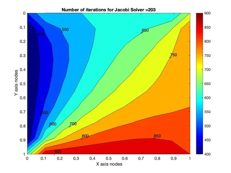
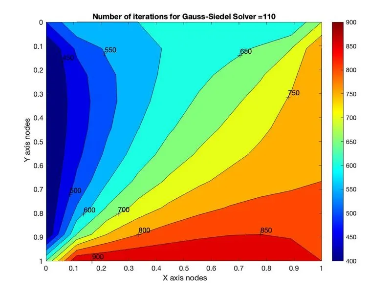
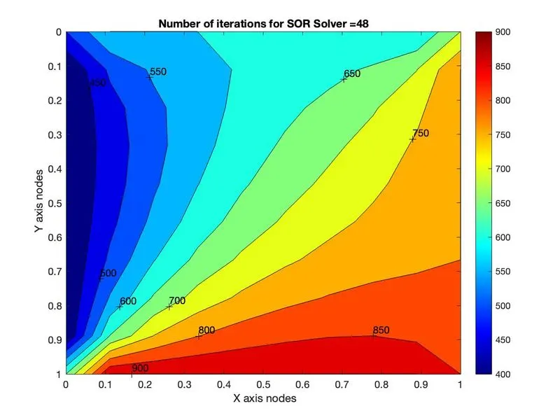
| Iterative Solver Technique | No. of iterations to reach SS |
|
Jacobi |
203 |
|
Gauss Siedel |
110 |
|
Successive Over-Relaxation |
48 |
Inference : From the steady state results, it can be inferred that the teamperatures at the nodes were the same for all the 3 different methodologies of iterative solvers. The solution at steady state were accurate, however the number of iterations needed to converge to steady state were significantly different between the 3 methods.
Jacobi took the longest time for convergence, whilst Gauss Siedel took comparitively lesser number of iterations (46% faster). This is mainly because Gauss siedel makes use of the solution of the previous nodes in the same timestep.
SOR was a variation of the Gauss Siedel that used a wighting parameter to converge to the solution faster. The weighing parameter that was used was 1.2 (w>1) to make it over-relaxed and hence the number of iterations needed to reach SS was reduced by 56% when compared to Gauss Siedel.
UnSteady State Solution :
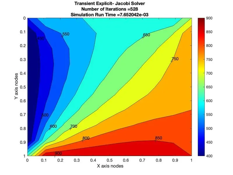
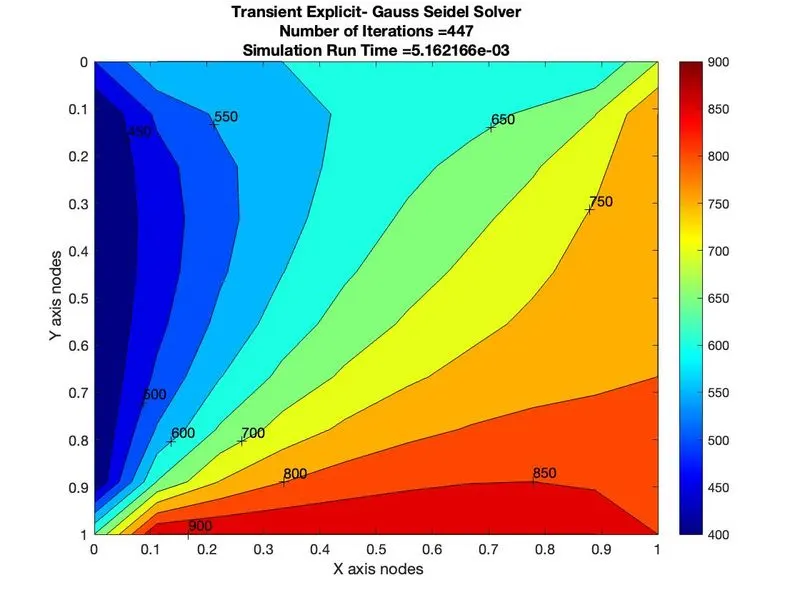
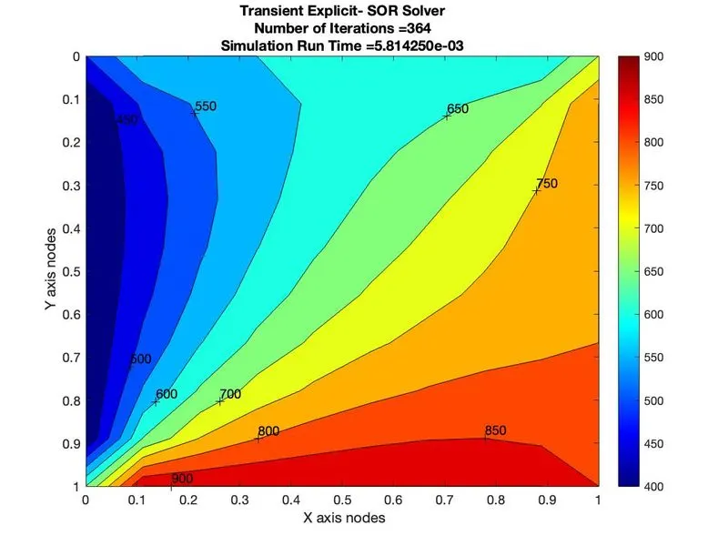
| Iterative Solver Technique (Implicit) | No. of iterations to reach |
|
Jacobi |
528 |
|
Gauss Siedel |
447 |
|
Successive Over-Relaxation |
364 |
Inference : It can be realized the explicit solution takes much lesser time when compared to implicit solution however the same trend can be observerved wherein Jacobi takes the longest to converge to a solution when compared to Gauss Sieldel and SOR methods.
-------------------------------------------------------------------------------------
Matlab Codes
Explicit Solution
clc
clear
close all

nx=10;
ny=nx;

x= linspace(0,1,nx);
y= linspace(0,1,nx);

dx= x(2)-x(1);
dy=dx;

Error=9e9;
tolerance=1e-4;

tT = 600;
tB = 900;
tL = 400;
tR = 800;

% Boundary conditions at Sides

T = 400*ones(nx,ny);
T(1,2:ny-1)= tT;
T(ny,2:ny-1)=tB;
T(2:nx-1,1)=tL;
T(2:nx-1,ny)=tR;

% Boundary conditions at Edges

T(1,1)= (T(1,2)+T(2,1))/2;
T(1,10)= (T(1,9)+T(2,10))/2;
T(10,1)=(T(9,1)+T(10,2))/2;
T(10,10)=(T(10,9)+T(9,10))/2;


T_initial = T;
T_Old = T ;

% Iterative Solvers

iterative_solver =1;
%% Jacobi ---- Iterative Solver1
% Jacobi Iterative Solver
k=2*((dx^2+dy^2)/(dx^2*dy^2));

if iterative_solver == 1
    jacobi_Iteration =1;

    while Error>tolerance
        for i= 2:nx-1
            for j=2:ny-1

                term1= (T_Old(i-1,j)+T_Old(i+1,j))/(k*(dx^2));
                term2= (T_Old(i,j-1)+T_Old(i,j+1))/(k*(dx^2));
                T(i,j) = term1+term2;
            end
        end

        Error = max(max(abs(T_Old-T)));
        T_Old=T;
        jacobi_Iteration = jacobi_Iteration+1;
    end


% Plotting

figure(1)
contourf(x,y,T)
clabel(contourf(x,y,T))
colorbar
colormap(jet)
set(gca, 'YDir','reverse')
xlabel(' X axis nodes');
ylabel(' Y axis nodes');
title(sprintf('Number of iterations for Jacobi Solver =%d',jacobi_Iteration));
pause(0.01)

end

%% Gauss-Siedel -- Iterative Solver2

if iterative_solver==2
    GS_Iteration =1;

    while Error>tolerance
        for i= 2:nx-1
            for j=2:ny-1

                term1= (T(i-1,j)+T_Old(i+1,j))/(k*(dx^2));
                term2= (T(i,j-1)+T_Old(i,j+1))/(k*(dx^2));
                T(i,j) = term1+term2;
            end
        end

        Error = max(max(abs(T_Old-T)));
        T_Old=T;
       GS_Iteration = GS_Iteration+1;
    end

 % Plotting

figure(2)
contourf(x,y,T)
clabel(contourf(x,y,T))
colorbar
colormap(jet)
set(gca, 'YDir','reverse')
xlabel(' X axis nodes');
ylabel(' Y axis nodes');
title(sprintf('Number of iterations for Gauss-Siedel Solver =%d',GS_Iteration));
pause(0.01)

end


%% Sucessive Over Relaxation (SOR) -- Iterative Solver3

alpha =1.7;
if iterative_solver==3
    SOR_Iteration =1;

    while Error>tolerance
        for i= 2:nx-1
            for j=2:ny-1

                term1= (T(i-1,j)+T_Old(i+1,j))/(k*(dx^2));
                term2= (T(i,j-1)+T_Old(i,j+1))/(k*(dx^2));
                GS(i,j) = term1+term2;
                T(i,j) = alpha* GS(i,j) + ((1-alpha)*T_Old(i,j));
            end
        end

        Error = max(max(abs(T_Old-T)));
        T_Old=T;
       SOR_Iteration = SOR_Iteration+1;
    end

 % Plotting

figure(2)
contourf(x,y,T)
clabel(contourf(x,y,T))
colorbar
colormap(jet)
set(gca, 'YDir','reverse')
xlabel(' X axis nodes');
ylabel(' Y axis nodes');
title(sprintf('Number of iterations for SOR Solver =%d',SOR_Iteration));
pause(0.01)

end
Implicit Solution:
clc
clear all
close all

nx=10;
ny=nx;
nt=1400;

x= linspace(0,1,nx);
y= linspace(0,1,nx);

dx= x(2)-x(1);
dy=dx;
dt=1e-3;
alpha =1.1;

Error=9e9;
tolerance=1e-4;

tT = 600;
tB = 900;
tL = 400;
tR = 800;


% Boundary conditions at Sides

T = 400*ones(nx,ny);
T(1,2:ny-1)= tT;
T(ny,2:ny-1)=tB;
T(2:nx-1,1)=tL;
T(2:nx-1,ny)=tR;

% Boundary conditions at Edges

T(1,1)= (T(1,2)+T(2,1))/2;
T(1,10)= (T(1,9)+T(2,10))/2;
T(10,1)=(T(9,1)+T(10,2))/2;
T(10,10)=(T(10,9)+T(9,10))/2;


T_initial = T;
T_Old = T ;

k1 = alpha*(dt/(dx^2));
k2 = alpha*(dt/(dy^2));

iterative_solver=1;

%% Jacobi Iterative Solver ==1 - Explicit solution

if iterative_solver==1

    jacobi_Iteration=1;
    tic

    for k=1:nt;

    while Error>tolerance
        for i= 2:nx-1
            for j=2:ny-1

                term1 = T_Old(i,j);
                term2 = k1*((T_Old(i-1,j))-(2*T_Old(i,j))+(T_Old(i+1,j)));
                term3 = k2*((T_Old(i,j-1))-(2*T_Old(i,j))+(T_Old(i,j+1)));

                T(i,j) = term1+term2+term3;
            end
        end

                 Error = max(max(abs(T_Old-T)));
        T_Old=T;
        jacobi_Iteration = jacobi_Iteration+1;

    end
        end


time_elapsed=toc;
    % Plotting

figure(1)
contourf(x,y,T)
clabel(contourf(x,y,T))
colorbar
colormap(jet)
set(gca, 'YDir','reverse')
xlabel(' X axis nodes');
ylabel(' Y axis nodes');
title1=sprintf('Number of Iterations =%d',jacobi_Iteration);
title2=sprintf('Simulation Run Time =%d',time_elapsed);
title({'Transient Explicit- Jacobi Solver';title1;title2});
pause(0.05)
end
%% GS Iterative Solver ==2 - Explicit solution

if iterative_solver==2

   GS_Iteration=1;
    tic

    for k=1:nt;

    while Error>tolerance
        for i= 2:nx-1
            for j=2:ny-1

                term1 = T_Old(i,j);
                term2 = k1*((T(i-1,j))-(2*T_Old(i,j))+(T_Old(i+1,j)));
                term3 = k2*((T(i,j-1))-(2*T_Old(i,j))+(T_Old(i,j+1)));

                T(i,j) = term1+term2+term3;
            end
        end

                 Error = max(max(abs(T_Old-T)));
        T_Old=T;
       GS_Iteration = GS_Iteration+1;

    end
        end


time_elapsed=toc;
    % Plotting

figure(1)
contourf(x,y,T)
clabel(contourf(x,y,T))
colorbar
colormap(jet)
set(gca, 'YDir','reverse')
xlabel(' X axis nodes');
ylabel(' Y axis nodes');
title1=sprintf('Number of Iterations =%d',GS_Iteration);
title2=sprintf('Simulation Run Time =%d',time_elapsed);
title({'Transient Explicit- Gauss Seidel Solver';title1;title2});
pause(0.05)

end

%% SOR Iterative Solver ==3 - Explicit solution

if iterative_solver==3
    omega=1.2;
   SOR_Iteration=1;
    tic

    for k=1:nt;

    while Error>tolerance
        for i= 2:nx-1
            for j=2:ny-1

                term1 = T_Old(i,j);
                term2 = k1*((T(i-1,j))-(2*T_Old(i,j))+(T_Old(i+1,j)));
                term3 = k2*((T(i,j-1))-(2*T_Old(i,j))+(T_Old(i,j+1)));

                GS(i,j) = term1+term2+term3;
                T(i,j) = omega* GS(i,j) + ((1-omega)*T_Old(i,j));
            end
        end

                 Error = max(max(abs(T_Old-T)));
        T_Old=T;
       SOR_Iteration = SOR_Iteration+1;

    end
        end


time_elapsed=toc;

% Plotting

figure(1)
contourf(x,y,T)
clabel(contourf(x,y,T))
colorbar
colormap(jet)
set(gca, 'YDir','reverse')
xlabel(' X axis nodes');
ylabel(' Y axis nodes');
title1=sprintf('Number of Iterations =%d',SOR_Iteration);
title2=sprintf('Simulation Run Time =%d',time_elapsed);
title({'Transient Explicit- SOR Solver';title1;title2});
pause(0.05)

end