Week 3.5 - Deriving 4th order approximation of a 2nd order derivative using Taylor Table method
Aim: To derive the fourth order approximation of the second order derivative using 3 numerical methods namely,
1) Central Differencing Scheme (CDS)
2) Skewed right-sided difference (FDS)
3) Skewed left-sided difference (BDS)
And to code the solution in Matlab to compare the absolute error from the analytical approach to compare the accuracy of these approaches.
Methodology:
Central Difference Scheme
To estimate the solution by CDS approach, 4 points are required being 2 points on the LHS and 2 points on the RHS of the function f(X).
Hence f(i-2dx) , f(i-dx),f(i), f(i+dx) and f(i+2dx) are required.
Therefore the second derivarive could be written as,
`(d^2u)/(dx^2) = (a.f(i-2)+b.f(i-1)+c.f(i)+d.f(i+1)+e.f(i+2))`
from the above equation, taylor's series can be derived and is shown below.
|
f(x) |
f’(x) Δx |
Δx2 f’’(x) |
Δx3 f’’’(x) |
Δx4 f’’’’(x) |
|
|
a.f (i-2) |
a |
-2a |
4a/2 |
-8a/6 |
16a/24 |
|
b.f (i-1) |
b |
-b |
b/2 |
-b/6 |
b/24 |
|
c.f (i) |
c |
0 |
0 |
0 |
0 |
|
d.f (i+1) |
d |
d |
d/2 |
d/6 |
d/24 |
|
e.f (i+2) |
e |
2e |
4e/2 |
8e/6 |
16e/24 |
|
Σ |
0 |
0 |
1 |
0 |
0 |
From the taylor's table , wee can get 5 equations with 5 unknowns
1) a+b+c+d+e = 0
2) (-2*a)-b+d+(2*e)= 0
3) (2*a)+(b/2)+(d/2)+(2*e)= 1
4) (-8*a/6)-(b/6)+(d/6)+(8*e/6) =0
5) (16*a/24)+(b/24)+(d/24)+(16*e/24)=0
Solving these equations could give the values of a,b,c,d and e.
a=-0.0833
b=1.3333
c=-2.5000
d=1.3333
e=-0.0833
Skewed right-sided difference (FDS)
To estimate the solution by CDS approach, 4 points to the right of the function are required
Hence f(i) , f(i+dx),f(i+2dx), f(i+3dx) and f(i+4dx) are required. Therefore the derivative could be written as,
`(d^2u)/(dx^2) = (a.f(i)+b.f(i+1)+c.f(i+2)+d.f(i+3)+e.f(i+4))`
Taylors series expansion of the above equation is used to populate the taylor's table as below,
|
f(x) |
f’(x) Δx |
Δx2 f’’(x) |
Δx3 f’’’(x) |
Δx4 f’’’’(x) |
|
|
a.f (i) |
a |
0 |
0 |
0 |
0 |
|
b.f (i+1) |
b |
b |
b/2 |
b/6 |
b/24 |
|
c.f (i+2) |
c |
2c |
4c/2 |
8c/6 |
16c/24 |
|
d.f (i+3) |
d |
3d |
4d/2 |
27d/6 |
81d/24 |
|
e.f (i+4) |
e |
4e |
16e/2 |
64e/6 |
256e/24 |
|
Σ |
0 |
0 |
1 |
0 |
0 |
From the taylor's table we can get 5 equations with 5 unknowns to solve for a,b,c,d and e.
1) a+b+c+d+e = 0
2) b+(2*c)+(3*d)+(4*e)=0
3) (b/2)+(2*c)+(9*d/2)+(8*e)=1
4) (b/6)+(8*c/6)+(27*d/6)+(64*e/6)=0
5) (b/24)+(16*c/24)+(81*d/24)+(256*e/24)=0
Solving these equations yield the values,
a=2.9167
b=-8.6667
c=9.5000
d=-4.6667
e=0.9167
Skewed left-sided difference (BDS)
To estimate the solution by CDS approach, 4 points to the left of the function are required
Hence f(i) , f(i-dx),f(i-2dx), f(i-3dx) and f(i-4dx) are required. Therefore the derivative could be written as,
`(d^2u)/(dx^2) = (a.f(i-4)+b.f(i-3)+c.f(i-2)+d.f(i-1)+e.f(i))`
Taylors series expansion of the above equation is used to populate the taylor's table as below,
|
f(x) |
f’(x) Δx |
Δx2 f’’(x) |
Δx3 f’’’(x) |
Δx4 f’’’’(x) |
|
|
a.f (i-4) |
a |
-4a |
16a/2 |
-64a/6 |
256a/24 |
|
b.f (i-3) |
b |
-3b |
9b/2 |
-27b/6 |
81b/24 |
|
c.f (i-2) |
c |
-2c |
4c/2 |
-8c/6 |
16c/24 |
|
d.f (i-1) |
d |
-d |
d/2 |
-d/6 |
d/24 |
|
e.f (i) |
e |
0 |
0 |
0 |
0 |
|
Σ |
0 |
0 |
1 |
0 |
0 |
From the taylor's table we can get 5 equations with 5 unknowns to solve for a,b,c,d and e.
1) a+b+c+d+e = 0
2) (-4*e)+(-3*d)+(-2*c)+(-1*b) = 0
3) (16*e/2)+(9*d/2)+(4*c/2)+(b/2)= 1
4) (-64*e/6)+(-27*d/6)+(-8*c/6)+(-b/6) = 0
5) (256*e/24)+(81*d/24)+(16*c/24)+(b/24) = 0
Solving the above equations results in,
a=2.9167
b=-8.6667
c=9.5000
d=-4.6667
e=0.9167
Results and Discussion
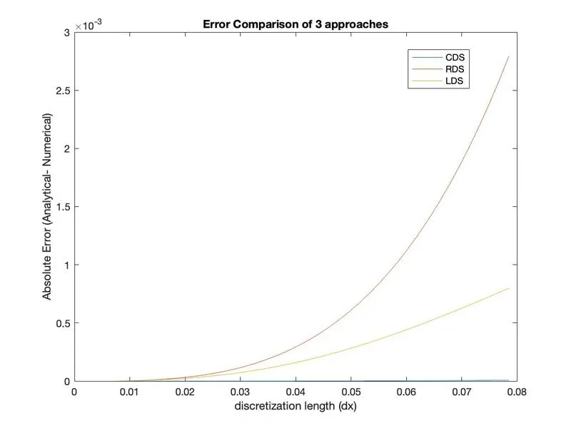
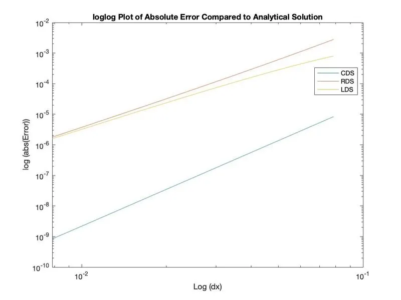
Inference :
It can be inferred from the above plots that the Central Differencing approach yields the least error and is the most accurate of the 3 methodologies that were compared. And it can also be restated from this assignment that discretization length also plays a significant role in error term reduction.
However the discretization length played a more pronounced role in the Skewed differencing approaches. Hence if a Right/Left side Skewed differencing approach is to be used, a smaller discretization length is preferred to ensure solution accuracy.
Advantages of a Skewed Scheme:
Though a Central difference scheme yields lesser error and is more accurate when compared to a Skewed approach, the CDS cannot always be used. For example if we consider the boundary or edge nodes of a domain, nodes to the right or left of the edges might nor be available to extract data from. Hence a it becomes a necessity to use a skewed approach to obtain the numerical solution.
Matlab Code
clc
clear
close all

%% Solving for coefficients by matrix inversion method

% Central difference scheme

syms a1 b1 c1 d1 e1

central_eq_1 = a1+b1+c1+d1+e1 == 0;
central_eq_2 = (-2*a1)-b1+d1+(2*e1)==0;
central_eq_3 = (2*a1)+(b1/2)+(d1/2)+(2*e1)==1;
central_eq_4 = (-8*a1/6)-(b1/6)+(d1/6)+(8*e1/6)==0;
central_eq_5 = (16*a1/24)+(b1/24)+(d1/24)+(16*e1/24)==0;

central_coeff= solve([central_eq_1,central_eq_2,central_eq_3,central_eq_4,central_eq_5],[a1,b1,c1,d1,e1]);

a1= double(central_coeff.a1);
b1= double(central_coeff.b1);
c1= double(central_coeff.c1);
d1= double(central_coeff.d1);
e1= double(central_coeff.e1);

% Right Skewed scheme

syms a2 b2 c2 d2 e2

right_eq_1 = a2+b2+c2+d2+e2 == 0;
right_eq_2 = b2+(2*c2)+(3*d2)+(4*e2)==0;
right_eq_3 = (b2/2)+(2*c2)+(9*d2/2)+(8*e2)==1;
right_eq_4 = (b2/6)+(8*c2/6)+(27*d2/6)+(64*e2/6)==0;
right_eq_5 = (b2/24)+(16*c2/24)+(81*d2/24)+(256*e2/24)==0;

right_coeff= solve([right_eq_1,right_eq_2,right_eq_3,right_eq_4,right_eq_5],[a2,b2,c2,d2,e2]);

a2= double(right_coeff.a2);
b2= double(right_coeff.b2);
c2= double(right_coeff.c2);
d2= double(right_coeff.d2);
e2= double(right_coeff.e2);

% Left Skewed scheme

syms a3 b3 c3 d3 e3

left_eq_1 = a3+b3+c3+d3+e3 == 0;
left_eq_2 = (-4*e3)+(-3*d3)+(-2*c3)+(-1*b3) == 0;
left_eq_3 = (16*e3/2)+(9*d3/2)+(4*c3/2)+(b3/2)== 1;
left_eq_4 = (-64*e3/6)+(-27*d3/6)+(-8*c3/6)+(-b3/6) == 0;
left_eq_5 = (256*e3/24)+(81*d3/24)+(16*c3/24)+(b3/24) == 0;

left_coeff= solve([left_eq_1,left_eq_2,left_eq_3,left_eq_4,left_eq_5],[a3,b3,c3,d3,e3]);

a3= double(left_coeff.a3);
b3= double(left_coeff.b3);
c3= double(left_coeff.c3);
d3= double(left_coeff.d3);
e3= double(left_coeff.e3);

%% Main Code

% f(x) = exp(x)*cos(x)

x=pi/3;
dx = linspace(pi/40,pi/400,40);

% Analytical solution
% f''(x) = -2*exp(x)*sin(x)

Analytical_solution = -2*exp(x)*sin(x);


for i= 1: length(dx)

% Taylor series terms

f_i_minus_4(i) = exp(x-(4*dx(i)))*cos(x-(4*dx(i)));
f_i_minus_3(i) = exp(x-(3*dx(i)))*cos(x-(3*dx(i)));
f_i_minus_2(i) = exp(x-(2*dx(i)))*cos(x-(2*dx(i)));
f_i_minus_1(i) = exp(x-(1*dx(i)))*cos(x-(1*dx(i)));
f_i(i)         = exp(x-(0*dx(i)))*cos(x-(0*dx(i)));
f_i_plus_1(i) = exp(x+(1*dx(i)))*cos(x+(1*dx(i)));
f_i_plus_2(i) = exp(x+(2*dx(i)))*cos(x+(2*dx(i)));
f_i_plus_3(i) = exp(x+(3*dx(i)))*cos(x+(3*dx(i)));
f_i_plus_4(i) = exp(x+(4*dx(i)))*cos(x+(4*dx(i)));


% Central differencing method


CDS_derivative(i) = ((a1*f_i_minus_2(i))+(b1*f_i_minus_1(i))+(c1*f_i(i))+(d1*f_i_plus_1(i))+(e1*f_i_plus_2(i)))/(dx(i)^2);
RDS_derivative(i) = ((a2*f_i(i))+(b2*f_i_plus_1(i))+(c2*f_i_plus_2(i))+(d2*f_i_plus_3(i))+(e2*f_i_plus_4(i)))/(dx(i)^2);
LDS_derivative(i) = ((a3*f_i(i))+(b3*f_i_minus_1(i))+(c3*f_i_minus_2(i))+(d3*f_i_minus_3(i))+(e3*f_i_minus_4(i)))/(dx(i)^2);

CDS_ERROR(i) = abs(Analytical_solution-CDS_derivative(i));
RDS_ERROR(i) = abs(Analytical_solution-RDS_derivative(i));
LDS_ERROR(i) = abs(Analytical_solution-LDS_derivative(i));

end

%% Plotting

figure(1)
loglog(dx,CDS_ERROR)
hold on
loglog(dx,RDS_ERROR)
hold on
loglog(dx,LDS_ERROR)
legend('CDS','RDS','LDS')

figure(2)
plot(dx,CDS_ERROR)
hold on
plot(dx,RDS_ERROR)
hold on
plot(dx,LDS_ERROR)
legend('CDS','RDS','LDS')

figure(3)
plot(f_i_minus_4)
hold on
plot(f_i_minus_3)
hold on
plot(f_i_minus_2)
hold on
plot(f_i_minus_1)
hold on
plot(f_i)