Simulation of a 1D Super-sonic nozzle flow simulation using MacCormack Method
Aim:
To stimulate Isentropic flow through a quasi 1D Subsonic-Supersonic nozzle by deriving the conservation and non-conservation forms of the governing equations and solving them using MacCormack's technique.
Isentropic Nozzle:
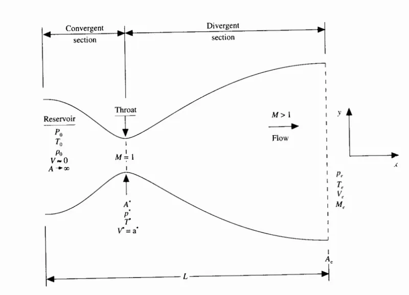
We are considering a steady-state, isentropic flow through a convergent-Divergent Nozzle. The flow at the inlet of the nozzle comes from a Reservoir. The cross-sectional area of the reservoir is large, and hence the velocity is very small. The flow expands isentropically to supersonic speeds at the nozzle exits. The flow is locally subsonic in the convergent section of the nozzle, sonic at the throat, and supersonic at the divergent section.
We are assuming that the flow properties vary only with x this is tantamount to assuming uniform flow properties across any given cross-section, Such flow is defined as Quasi one-dimensional flow.
Conservative form:
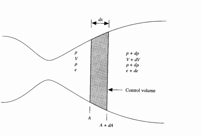
Conservation form or Eulerian form refers to an arrangement of an equation or system of equations, Where the Control volume is Constant.
Non-Conversative form:
Conservation form or Eulerian form refers to an arrangement of an equation or system of equations, Where the Control volume is moving.
General form of Govering equation for quasi one dimensional ,steady, Isentropic flow:
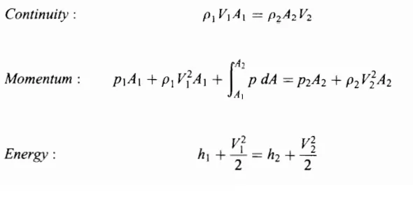
Non-Conservative form of governing equations:
Continuity equation:

Momentum equation:

Energy Equation:

Conversative form of Governing equation:
Continuity Equation:
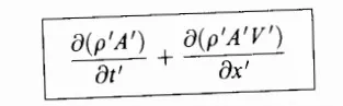
Momentum Equation:
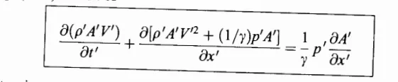
Energy Equation:

Boundary Condition:
Conservative form:
Inlet:
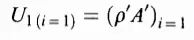

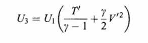
Outlet:
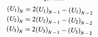
Non Conversative form:
inlet
v(1)=2*v(2)-v(3);
outlet
v(n)=2*v(n-1)-v(n-2);
rho(n)=2*rho(n-1)-rho(n-2);
t(n)=2*t(n-1)-t(n-2);
Program:
Main Code:
clear all
close all
clc

%inputs
n=31;
x=linspace(0,3,n);
dx=x(2)-x(1);
gamma=1.4;

%calling function:
 [rho_nc,v_nc,t_nc,mass_flow_nc,p_nc,mach_nc,v_throat_nc,p_throat_nc,rho_throat_nc,mass_flow_nt_nc,mach_nt_nc,t_throat_nc]=nonconversative(n,x,dx,gamma);

 [rho_c,v_c,t_c,mass_flow_c,p_c,mach_c,v_throat_c,p_throat_c,rho_throat_c,mass_flow_nt_c,mach_nt_c,t_throat_c]=conversative(n,x,dx,gamma);


%plotting
figure(1)
subplot(4,1,1)
plot(x,t_c,'linewidth',2,'color','r')
hold on
plot(x,t_nc,'linewidth',2,'color','b')
xlabel('length of the Nozzle')
ylabel('Temperature')
title({'Flow paramters throughout the length of the nozzle (Conservative)';'Length of the nozzle vs Temperature'})
legend({'Conservative','Non-conservative'})
subplot(4,1,2)
hold on
plot(x,rho_c,'linewidth',2,'color','r')
plot(x,rho_nc,'linewidth',2,'color','b')
xlabel('length of the Nozzle')
ylabel('Density')
title('Length of the nozzle vs Density')
legend({'Conservative','Non-conservative'})
subplot(4,1,3)
hold on
plot(x,v_c,'linewidth',2,'color','r')
plot(x,v_nc,'linewidth',2,'color','b')
xlabel('length of the Nozzle')
ylabel('Velocity')
title('Length of the nozzle vs velocity')
legend({'Conservative','Non-conservative'})
subplot(4,1,4)
hold on
plot(x,p_c,'linewidth',2,'color','r')
plot(x,p_nc,'linewidth',2,'color','b')
xlabel('length of the Nozzle')
ylabel('Pressure')
title('Length of the nozzle vs Pressure')
legend({'Conservative','Non-conservative'})


figure(2)
hold on
plot(x,mach_c,'color','c');
plot(x,mach_nc,'color','r');
xlabel('length of the Nozzle')
ylabel('mach')
title({'Normalized mass flow rate(Conservative)';'Length of the nozzle vs velocity'})
legend({'Conservative','Non-conservative'})

figure(3)
hold on
plot(x,mass_flow_c,'color','c')
plot(x,mass_flow_nc,'color','r')
xlabel('Length of the Nozzle')
ylabel('Mass flow rate')
title('Length of the Nozzle vs Mass flow rate')
legend({'Conservative','Non-conservative'})

figure(4)
subplot(4,1,1)
hold on
plot(t_throat_c,'color','b')
plot(t_throat_nc,'color','g')
title({'Time-Wise variation';'Time steps vs Temperature'})
xlabel('Time steps')
ylabel('Temperature')
legend({'Conservative','Non-conservative'})
subplot(4,1,2)
hold on
plot(rho_throat_c,'color','b')
plot(rho_throat_nc,'color','g')
title({'Time-Wise variation';'Time steps vs Density'})
xlabel('Time steps')
ylabel('Density')
legend({'Conservative','Non-conservative'})
subplot(4,1,3)
hold on
plot(v_throat_c,'color','b')
plot(v_throat_nc,'color','g')
title({'Time-Wise variation';'Time steps vs Velocity'})
xlabel('Time steps')
ylabel('Velocity')
legend({'Conservative','Non-conservative'})
subplot(4,1,4)
hold on
plot(p_throat_c,'color','b')
plot(p_throat_nc,'color','g')
title({'Time-Wise variation';'Time steps vs Pressure'})
xlabel('Time steps')
ylabel('Pressure')
legend({'Conservative','Non-conservative'})
Non-Conservative form:
function [rho,v,t,mass_flow,p,mach,v_throat,p_throat,rho_throat,mass_flow_nt,mach_nt,t_throat] = nonconversative(n,x,dx,gamma)

%calculate initial profiles
rho=1-0.3146*x;
%temperature
t=1-0.2314*x;
v=(0.1+1.09*x).*t.^0.5;
%area
a=1+2.2*(x-1.5).^2;
throat=find(a==1);

%Time loops
nt=1400;
dt=0.0201; %Value used in anderson ch.7 for non-cons.form

%outer time loop

for k=1:nt

    rho_old=rho;
    v_old=v;
    t_old=t;

   %Predicted method:

    for j=2:n-1
        dvdx=(v(j+1)-v(j))/dx;
        drhodx=(rho(j+1)-rho(j))/dx;
       % dtdx=(t(j+1)-(j))/dx;
         dtdx=(t(j+1)-t(j))/dx;
        dlogadx=(log(a(j+1))-log(a(j)))/dx;

        %Continuity equation

        drhodt_p(j)=-rho(j)*dvdx-rho(j)*v(j)*dlogadx-v(j)*drhodx;

        %Momentum equation

      %  dvdt_p(j)=-v(j)*dvdx-(1/gamma)*(dt/dx+(t(j)/rho(j))*drhodx);
         dvdt_p(j)=-v(j)*dvdx-(1/gamma)*(dtdx+(t(j)/rho(j))*drhodx);
        %Energy equation

        dtdt_p(j)=-v(j)*dtdx-(gamma-1)*t(j)*(dvdx+v(j)*dlogadx);

    end
      % solution update:
     for i=2:n-1
        v(i) = v(i) + dvdt_p(i)*dt;
        t(i) = t(i) + dtdt_p(i)*dt;
        rho(i) = rho(i) + drhodt_p(i)*dt;
     end

    %Corrected method:
     for l=2:n-1

        dvdx=(v(l)-v(l-1))/dx;
        drhodx=(rho(l)-rho(l-1))/dx;
       % dtdx=(t(l)-(l-1))/dx;
        dtdx=(t(l)-t(l-1))/dx;
        dlogadx=(log(a(l))-log(a(l-1)))/dx;

        %Continuity equation:
        drhodt_c(l)=-rho(l)*dvdx-rho(l)*v(l)*dlogadx-v(l)*drhodx;

        %Momentum equation:
       % dvdt_c(l)=-v(l)*dvdx-(1/gamma)*(dt/dx+(t(l)/rho(l))*drhodx);
       dvdt_c(l)=-v(l)*dvdx-(1/gamma)*(dtdx+(t(l)/rho(l))*drhodx);

        %Energy equation
        dtdt_c(l)=-v(l)*dtdx-(gamma-1)*t(l)*(dvdx+v(l)*dlogadx);

     end

    %Compute the average time derivative:

     drhodt=0.5*(drhodt_p+drhodt_c);
     dvdt=0.5*(dvdt_p+dvdt_c);
     dtdt=0.5*(dtdt_p+dtdt_c);

     %Final solution update:
     for i=2:n-1
        v(i) = v_old(i) + dvdt(i)*dt;
        t(i) = t_old(i) + dtdt(i)*dt;
        rho(i) = rho_old(i) + drhodt(i)*dt;
     end

    %Applying the boundary condtitions

    %inlet
    v(1)=2*v(2)-v(3);
    %outlet
    v(n)=2*v(n-1)-v(n-2);
    rho(n)=2*rho(n-1)-rho(n-2);
    t(n)=2*t(n-1)-t(n-2);

%Mass flow rate:
mass_flow=rho.*a.*v;
%Pressure:
p=rho.*t;
%Mach_no:
mach=(v./sqrt(t));

%Calculating variables at throat:
t_throat(k)=t(throat);
rho_throat(k)=rho(throat);
p_throat(k)=p(throat);
mass_flow_nt(k)=mass_flow(throat);
mach_nt(k)=mach(throat);
v_throat(k)=v(throat);


figure(5)
if k ==50
    plot(x,mass_flow,'m','linewidth',2)
    hold on
elseif k ==100
    plot(x,mass_flow,'c','linewidth',2)
    hold on
elseif k==500
    plot(x,mass_flow,'g','linewidth',2)
    hold on
elseif k==700
    plot(x,mass_flow,'r','linewidth',2)
    hold on
elseif k==1400
    plot(x,mass_flow,'b','linewidth',2)
    hold on
end
title('Variation of Mass flow rate distribution inside the nozzle(Non Conservative')
xlabel('Length of the Nozzle')
ylabel('Mass flow')
grid on
end
legend({'50 timestep','100 timestep','500 timestep','700 timestep','1400timestep'})

end
Conservative form:
function [rho,v,t,mass_flow,p,mach,v_throat,p_throat,rho_throat,mass_flow_nt,mach_nt,t_throat] = conversative(n,x,dx,gamma)

%inputs
nt=1400;
%Initial profiles for Density and Pressure
for i=1:n
    if(x(i)<=0.5)
        rho(i)=1.0;
        t(i)=1.0;
    end
    if(x(i)>=0.5&&x(i)<1.5)
        rho(i)=1.0-0.366*(x(i)-0.5);
        t(i)=1.0-0.167*(x(i)-0.5);
    end
    if(x(i)>=1.5&&x(i)<3.5)
        rho(i)=0.634-0.3879*(x(i)-1.5);
        t(i)=0.833-0.3507*(x(i)-1.5);
    end
end
%area
a=1+2.2*(x-1.5).^2;
throat=find(a==1);
%velocity
v=0.59./(rho.*a);
%Mass flow rate:
mass_flow=rho.*a.*v;
%Pressure:
p=rho.*t;
%Mach_no:
mach=(v./sqrt(t));

%Initial Solution
u1=rho.*a;
u2=u1.*v;
u3=u1.*((t/(gamma-1))+((gamma/2)*(v).^2));

dt = 0.0276;

for k = 1:nt

    %saving old values
    u1_old=u1;
    u2_old=u2;
    u3_old=u3;

    %Pure form of Flux vector (RHS to be only of source terms)
    f1 = u2;
    f2 = (u2.^2./u1)+((gamma-1)/gamma)*(u3-(gamma/2)*(u2.^2./u1));
    f3 = (gamma*((u2.*u3)./u1))-(((gamma*(gamma-1))/2)*(u2.^3./u1.^2));

    % PREDICTOR STEP:
    for j=2:n-1

    %Pure form of source term
   % j2=((gamma-1)/gamma)*(u3-(gamma/2)*(u2.^2./u1))*((log(a_c(j+1))-log(a_c(j)))/dx);
     j2 = (1/gamma)*rho(j)*t(j)*(a(j+1)-a(j))/dx;


    %continuity equation:
    du1_dt_p(j)=-(f1(j+1)-f1(j))/dx;
    %Momentum equation:
    du2_dt_p(j)=-((f2(j+1)-f2(j))/dx)+j2; %(j) for j2
    %Energy equation:
    du3_dt_p(j)=-(f3(j+1)-f3(j))/dx;

    %Solution update:
    u1(j)=u1(j)+du1_dt_p(j)*dt; %No old terms
    u2(j)=u2(j)+du2_dt_p(j)*dt;
    u3(j)=u3(j)+du3_dt_p(j)*dt;

    end

    %Updating flux terms
    f1 = u2;
    f2 = (u2.^2./u1)+((gamma-1)/gamma)*(u3-(gamma/2)*(u2.^2./u1));
    f3 = (gamma*((u2.*u3)./u1))-(((gamma*(gamma-1))/2)*(u2.^3./u1.^2));

    % For j2
    rho = u1./a;
    t = (gamma-1)*(u3./u1)-(gamma/2)*(u2./u1).^2;

    % CORRECTOR STEP
    for j =2:n-1

    %Pure form of source term
    %j2=((gamma-1)/gamma)*(u3-(gamma/2)*(u2.^2./u1))*((log(a(j))-log(a(j-1)))/dx);
    j2 = (1/gamma)*rho(j)*t(j)*(a(j)-a(j-1))/dx;

    %Corrected method
    %continuity equation:
    du1_dt_c(j)=-(f1(j)-f1(j-1))/dx;

    %Momentum equation:
    du2_dt_c(j)=-((f2(j)-f2(j-1))/dx)+j2; %No (j) for j2

    %Energy equation:
    du3_dt_c(j)=-(f3(j)-f3(j-1))/dx;

    end

%Computing average time derivative:

du1_dt=0.5*(du1_dt_p+du1_dt_c);
du2_dt=0.5*(du2_dt_p+du2_dt_c);
du3_dt=0.5*(du3_dt_p+du3_dt_c);

%Final solution update:
for l=2:n-1
    u1(l)=u1_old(l)+du1_dt(l)*dt;
    u2(l)=u2_old(l)+du2_dt(l)*dt;
    u3(l)=u3_old(l)+du3_dt(l)*dt;
end


%Applying boundary condition:

 %at inlet
   u1(1) = a(1);
   u2(1) = 2*u2(2)-u2(3);
   v(1) = u2(1)/u1(1);
   u3(1) = u1(1)*(t(1)/(gamma-1))+(gamma/2)*v(1)*2;

   %at outlet
   u1(n) = 2*u1(n-1)-u1(n-2);
   u2(n) = 2*u2(n-1)-u2(n-2);
   u3(n) = 2*u3(n-1)-u3(n-2);

    rho = u1./a;
    v = u2./u1;
    t = (gamma-1)*(u3./u1)-(gamma/2)*(u2./u1).^2;

%Mass flow rate:
mass_flow=rho.*a.*v;
%Pressure:
p=rho.*t;
%Mach_no:
mach=(v./sqrt(t));


%Calculating variables at throat:
t_throat(k)=t(throat);
rho_throat(k)=rho(throat);
p_throat(k)=p(throat);
mass_flow_nt(k)=mass_flow(throat);
mach_nt(k)=mach(throat);
v_throat(k)=v(throat);

figure(6)
if k ==50
    plot(x,mass_flow,'m','linewidth',2)
    hold on
elseif k ==100
    plot(x,mass_flow,'c','linewidth',2)
    hold on
elseif k==500
    plot(x,mass_flow,'g','linewidth',2)
    hold on
elseif k==700
    plot(x,mass_flow,'r','linewidth',2)
    hold on
elseif k==1400
    plot(x,mass_flow,'b','linewidth',2)
    hold on
end
title('Variation of Mass flow rate distribution inside the nozzle(Conservative')
xlabel('Length of the Nozzle')
ylabel('Mass flow')
grid on

end
legend({'50 timestep','100 timestep','500 timestep','700 timestep','1400timestep'})

end
Plots:
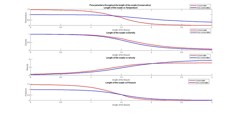
From the above plot, We can compare the primitive variables of Conservative and Non-Conservative form ie. Pressure, Temperature, Velocity, Density changes through the length of the nozzle.
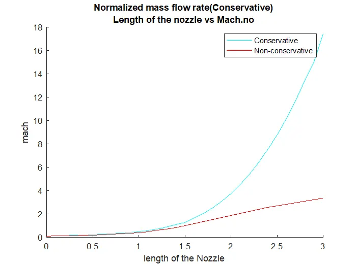
Mach No. is a dimensionless quantity in fluid dynamics representing the ratio of flow velocity past a boundary to the local speed of sound.
From the above plot, we can say that the Mach No. for the conservative form is greater than the non-conversation form, so the nozzle with higher Mach no. has higher efficiency.
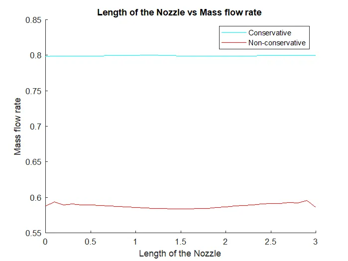
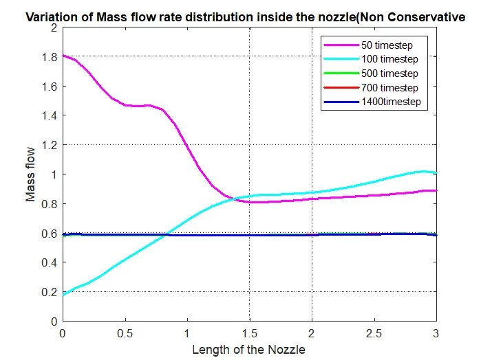
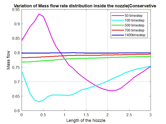
Mass flow rate is defined as the rate of movement of liquid pass through a unit area.
From the above plot, the Conservative form travels faster than Nonconservative form.
Conclusion:
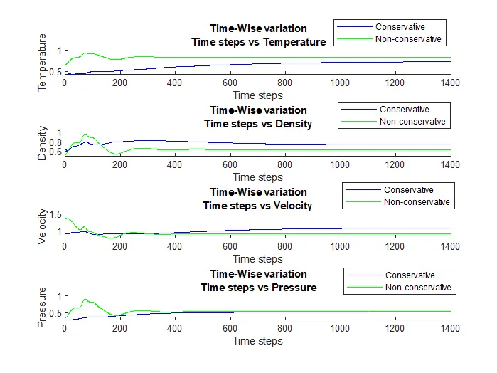
In this project, we learned about Isentropic flow through quasi-one-dimensional subsonic-Supersonic nozzle and the behavior of Temperature, Pressure, Velocity, Density, Mach No. and, Mass flow rate inside the nozzle by using the MacCormack method.