Week 7 - Simulation of a 1D Super-sonic nozzle flow simulation using Macormack Method
Objective: To simulate the isentropic flow through a quasi 1D subsonic-supersonic nozzle.
To plot:
1. Steady-state distribution of primitive variables inside the nozzle
2. Time-wise variation of the primitive variables
3. Variation of Mass flow rate distribution inside the nozzle at different time steps during the time-marching process
4. Comparison of Normalized mass flow rate distributions of both forms
Non-Dimensionalising the values:
First, we going to non-dimensionalize the flow field variable for the aesthetic advantage of presenting results. The non-dimensionalized
variables are given by,
`x' = x/L`
`rho' = rho/rho^o`
`T' = T/T^o`
`V' = V/a_o`
`t'= t/(L/a_o)`
`P=P/P^0`
`A'= A/A^"*"`
where,
L = Length of the nozzle
`T^o , rho^o , P^o` = temperature, density and pressure at stagnation condition respectevely
`a_o = sqrt(gamma R T_o)`
and `A^"*"` = throat area
MacCormack Method
MacCormack method is a discretization technique which is an explicit finite difference technique that is second-order accurate in space and time. The techniques make use of two first-order accurate schemes namely predictor step and corrector step and effectively make them second-order accurate.
Step 1: Predictor Step
In this step, we use foreward differencing schemes for spatial derivatives and calculate the solution
`((delf)/(dt))_p = (f(i+1) - f(i))/(Deltax)`
Solution update (Intermediate solution)
Step 2: Corrector Step
In this step, we use backward differencing schemes for spatial derivatives and calculate the solution gradient by which we reach an corrected
solution.
`((delf_p)/(dt))_c = (f(i) - f(i-1))/(Deltax)`.
Step 3: Final Solution
With use of two computed solution gradients ( predictor and colllector), we take the average of both and reach final solution.
`((delf)/(dt))_(avg) = 0.5(((delf)/(dt))_p +((delf_p)/(dt))_c )`
Final solution updated by adding the average to the initial state.
`f_(sol) = f_(Initial) + ((delf)/(delt))_(avg) * Deltat`
`f_(sol)`= Final solution of the flow field variable for the first time step
Matlab Code:
Main Code:
clear all
close all
clc


%heat capacity ratio
    gamma = 1.4;
%length
    L = 3;
%length of nozzle
    X = linspace(0,L,31);
    dx = X(2)-X(1);

%Calling function to save values of mass flow
    [m_nonconservative] = non_conservative(gamma,X,dx);
    [ m_Conservative] = Conservative(gamma,X,dx);
%To compare steady state mass flow for conservative and non conservative form
    figure(7)
    plot(X,m_nonconservative,'linewidth',2)
    hold on
    plot(X,m_Conservative,'linewidth',2)
    xlabel('Nozzle length')
    ylabel('Mass flow rate')
    legend('Non Conservative','Conservative');
    title('Massflow conservative and Non conservative form')
Function Code:(NON CONSERVATIVE)
function [m_plot] = non_conservative(gamma,X,dx)
%Initial condition
    rho = (1-0.3146*X);
    T = (1-0.2314*X);
    V = (0.1+1.09*X).*T.^0.5;
    A = 1+2.2*(X-1.5).^2;

%Speedof sound
a_initial = T.^0.5;
%Courant number
C = 0.5;
%time step calculation
delt = min(C*dx./(T.^0.5+V));


nt = 1400;
plot_no = 1;
iterno = 200;
for i = 1:nt
    %time step calculation
    delt = min(C*dx./(T.^0.5+V));

    for j = 2:length(X)-1


    term_a = (V(j+1)-V(j))/dx;
    term_b = (log(A(j+1))-log(A(j)))/dx;
    term_c = (rho(j+1)-rho(j))/dx;
    term_d = (T(j+1)-T(j))/dx;
%predictor
    %density
    drho_dt_predict(j) = -rho(j)*term_a- rho(j)*V(j)*term_b-V(j)*term_c;
    %Velocity
    dv_dt_predict(j) = -V(j)*term_a-(1/gamma)*(term_d+(T(j)/rho(j))*term_c);
    %Temperature
    dT_dt_predict(j) = -V(j)*(term_d)-(gamma-1)*T(j)*(term_a+V(j)*term_b);
%New predicted
    %rho
    rho_predict(j) = rho(j)+ drho_dt_predict(j)*delt;
    %Velocity
    V_predict(j) = V(j) + dv_dt_predict(j)*delt;
    %Temperature
    T_predict(j) = T(j) + dT_dt_predict(j)*delt;
    end
    rho_predict(1) = rho(1);
    V_predict(1) = V(1);
    T_predict(1) = T(1);


%<<<<<<<<<<<<<<<<<<<<<<<<<<<<<<<<<<<<Corrector>>>>>>>>>>>>>>>>>>>>>>>>>>>>>>>>>>>>>>>>>>>>>>>>>>
for j = 2:length(X)-1
    term_a = (V_predict(j)-V_predict(j-1))/dx;
    term_b = (log(A(j))-log(A(j-1)))/dx;
    term_c = (rho_predict(j)-rho_predict(j-1))/dx;
    term_d = (T_predict(j)-T_predict(j-1))/dx;

    %density
    drho_dt_correct(j) = -rho_predict(j)*term_a-rho_predict(j)*V_predict(j)*term_b-V_predict(j)*term_c;
    %Velocity
    dv_dt_correct(j) = -V_predict(j)*term_a-(1/gamma)*(term_d+(T_predict(j)/ rho_predict(j))*term_c);
    %Temperature
    dT_dt_correct(j) = -V_predict(j)*(term_d)-(gamma-1)*T_predict(j)*(term_a+V_predict(j)*term_b);
end
%<<<<<<<<<<<<<<<<<<<<<<<<<<<<<<<<<<<<New time step value computing>>>>>>>>>>>>>>>>>>>>>>>>>>>>>
for j = 2:length(X)-1

    rho_new(j-1) = rho(j)+ ((drho_dt_predict(j) + drho_dt_correct(j))/2)*delt;
    V_new(j-1) = V(j) + ((dv_dt_predict(j) + dv_dt_correct(j))/2)*delt;
    T_new(j-1) = T(j) + ((dT_dt_predict(j) + dT_dt_correct(j))/2)*delt;

end
%Assigning values of old timestep to new one
    rho(2:length(X)-1) = rho_new;
    V(2:length(X)-1) = V_new;
    T(2:length(X)-1) = T_new;
%Assigning boundary conditions
    %Inlet
    rho(1) = rho(1);
    V(1) = 2*V(2)-V(3);
    T(1) = T(1);
    %Outlet
    rho(length(X)) = 2*rho(length(X)-1)-rho(length(X)-2);
    V(length(X)) = 2*V(length(X)-1)-V(length(X)-2);
    T(length(X)) = 2*T(length(X)-1)-T(length(X)-2);
%<<<<<<<<<<<<<<<<<<<<<<<<<<<<<<<<<<<<savnig the throat velocity>>>>>>>>>>>>>>>>>>>>>>>>>>>>>>>>>
   plot_rho(i) = rho(16);
   plot_V(i) = V(16);
   plot_T(i) = V(16);
%To compute the mass flow rate at intermediate iterations
   if i == iterno
   m(plot_no,:) = rho.*A.*V;
   iterno = iterno+300;
   plot_no = plot_no+1;
   end

end

%Mass flow rate calculation
m_plot = rho.*A.*V;
%Mach number calculation
M = V./T.^0.5;

 figure(1)
 plot(X,m,'linewidth',2)
 xlabel('Nozzle length')
 ylabel('Mass flow rate')
 legend('Iteration NO: 200','Iteration NO: 500'...
            ,'Iteration NO: 800','Iteration NO: 1100','Iteration NO: 1400')
title('Massflow Non conservative form at different iteration')
%Iteration vs throat properties
figure(2)
subplot(3,1,1)
plot(plot_V);
title('Velocity')
xlabel('Number of time step')
ylabel('\bf{\it{V/a_0}}')
subplot(3,1,2)
plot(plot_T);
title('Temperature')
xlabel('Number of time step')
ylabel('\bf{\it{T/T_0}}')
subplot(3,1,3)
plot(plot_rho);
title('Density')
xlabel('Number of time step')
ylabel('\bf{\rho/\rho_0}')

%Variation of properties with nozzle distance
figure(3)
subplot(4,1,1)
plot(X,V);
title('Velocity')
xlabel('Non dimensional nozzle distance')
ylabel('\bf{\it{V/a_0}}')
subplot(4,1,2)
plot(X,T);
title('Temperature')
xlabel('Non dimensional nozzle distance')
ylabel('\bf{\it{T/T_0}}')
subplot(4,1,3)
plot(X,rho);
title('Density')
xlabel('Non dimensional nozzle distance')
ylabel('\bf{\rho/\rho_0}')
subplot(4,1,4)
plot(X,M);
title('Mach No.')
xlabel('Non dimensional nozzle distance')
ylabel('\bf{M}')

end
Function Code:(CONSERVATIVE)
function [ m_steadystate] = Conservative(gamma,X,dx)
%Initial conditions
for i = 1:length(X)
    if (0<=X(i) && X(i)<=0.5)
    rho(i) = 1;
    T(i) = 1;
    elseif (0.5<=X(i) && X(i)<=1.5)
    rho(i) = 1-0.366*(X(i)-0.5);
    T(i) = 1-0.167*(X(i)-0.5);
    elseif(1.5<=X(i) && X(i)<=3.5)
    rho(i) = 0.634-0.3879*(X(i)-1.5);
    T(i) = 0.833-0.3507*(X(i)-1.5);
    end
end

%Area variation
    A = 1+2.2*(X-1.5).^2;
%Velocity VRItion
    V = 0.59./(rho.*A);
    %Courant number
    C = 0.5;
%time step calculation
    delt = min(C*dx./(T.^0.5+V));
plot_no = 1;
iterno = 200;
 for i = 1:1400
%%
%Updating value of time step
   delt = min(C*dx./(T.^0.5+V));

%Solution Vector
    U_1 = rho.*A;
    U_2 = rho.*A.*V;
    U_3 = rho.*A.*((T./(gamma-1))+(gamma/2*V.^2));
%Flux Vector
    F_1 = U_2;
    F_2 = U_2.^2./U_1+((gamma-1)/gamma)*(U_3-(gamma/2)*(U_2.^2./U_1));
    F_3 = ((gamma*U_2.*U_3)./U_1)-((gamma*(gamma-1)/2)*(U_2.^3./U_1.^2));

%Updating value of predicted U_1,U_2and U_3
    U_1_predict = U_1;
    U_2_predict = U_2;
    U_3_predict = U_3;
% Space loop
    for j = 2:length(X)-1
%%
%<<<<<<<<<<<<<<<<<<<<<<<<<<<<<<<<<<<<<Predictor Step>>>>>>>>>>>>>>>>>>>>>>>>>>>>>>>>>>>>>>>>>>>>
%Source term
        J(j) = (1/gamma)*rho(j)*T(j)*(A(j+1)-A(j))/dx;

%Predictor values
        dU_1_dt_predict(j) = -(F_1(j+1)-F_1(j))/dx;
        dU_2_dt_predict(j) = -(F_2(j+1)-F_2(j))/dx+J(j);
        dU_3_dt_predict(j) = -(F_3(j+1)-F_3(j))/dx ;

        U_1_predict(j) = U_1(j)+ dU_1_dt_predict(j)*delt;
        U_2_predict(j) = U_2(j)+ dU_2_dt_predict(j)*delt;
        U_3_predict(j) = U_3(j)+ dU_3_dt_predict(j)*delt;

    end
%%
%Finding Predicted velocity density and temperature
    %density
    rho = U_1_predict./A;
    %Velocity
    V = U_2_predict./U_1_predict;
    %Temperature
    T = (gamma-1)*((U_3_predict./U_1_predict)-(gamma/2)*(V).^2);

%Updating values of F_1 F_2 and  F_3
    F_1 = U_2_predict;
    F_2 = U_2_predict.^2./U_1_predict+((gamma-1)/gamma)*(U_3_predict-(gamma/2)*(U_2_predict.^2./U_1_predict));
    F_3 = ((gamma*U_2_predict.*U_3_predict)./U_1_predict)-((gamma*(gamma-1)/2)*(U_2_predict.^3./U_1_predict.^2));

%%
%<<<<<<<<<<<<<<<<<<<<<<<<<<<<<<<<<<<<<Corrector Step>>>>>>>>>>>>>>>>>>>>>>>>>>>>>>>>>>>>>>>>>>>>
 for j = 2:(length(X)-1)
    J(j) = (1/gamma)*rho(j)*T(j)*(A(j)-A(j-1))/dx;
    dU_1_dt_correct(j) = -(F_1(j)-F_1(j-1))/dx;
    dU_2_dt_correct(j) = -(F_2(j)-F_2(j-1))/dx+ J(j);
    dU_3_dt_correct(j) = -(F_3(j)-F_3(j-1))/dx ;
end
%Averaging Step
    dU_1_dt = 0.5*(dU_1_dt_predict+dU_1_dt_correct);
    dU_2_dt = 0.5*(dU_2_dt_predict+dU_2_dt_correct);
    dU_3_dt = 0.5*(dU_3_dt_predict+dU_3_dt_correct);
%%
%new value of solution vector
for j = 2:(length(X)-1)
%Final step
    U_1_new(j) = U_1(j)+ dU_1_dt(j)*delt;
    U_2_new(j) = U_2(j)+ dU_2_dt(j)*delt;
    U_3_new(j) = U_3(j)+ dU_3_dt(j)*delt;
end

% Boundary condition-inlet
    U_1_new(1)=rho(1)*A(1);
    U_2_new(1)=(2*U_2_new(2))-U_2_new(3);
    U_3_new(1)=U_1_new(1)*(T(1)/(gamma-1)+(gamma/2)*V(1)^2);
% Boundary condition-outlet
    U_1_new(length(X))=2*U_1_new(length(X)-1)-U_1_new(length(X)-2);
    U_2_new(length(X))=2*U_2_new(length(X)-1)-U_2_new(length(X)-2);
    U_3_new(length(X))=2*U_3_new(length(X)-1)-U_3_new(length(X)-2);

%%
%New Value of Primitive variables
    rho = U_1_new./A;
    V = U_2_new./U_1_new;
    T = (gamma-1)*((U_3_new./U_1_new)-(gamma/2)*V.^2);
    M = V./T.^0.5;

%To compute the mass flow rate at intermediate iterations
    if i == iterno
    m(plot_no,:) = rho.*A.*V;
    iterno = iterno+300;
    plot_no = plot_no+1;
    end
    plot_rho(i) = rho(16);
    plot_V(i) = V(16);
    plot_T(i) = V(16);
 end
 m_steadystate = rho.*A.*V;
 %Plotting
 figure(4)
 plot(X,m,'linewidth',2)
 xlabel('Nozzle length')
 ylabel('Mass flow rate')
 legend('Iteration NO: 200','Iteration NO: 500'...
            ,'Iteration NO: 800','Iteration NO: 1100','Iteration NO: 1400')
 title('Massflow title Conservative form at different time step')


 %Iteration vs throat properties
figure(5)
subplot(3,1,1)
plot(plot_V);
title('Velocity')
xlabel('Number of time step')
ylabel('\bf{\it{V/a_0}}')
subplot(3,1,2)
plot(plot_T);
title('Temperature')
xlabel('Number of time step')
ylabel('\bf{\it{T/T_0}}')
subplot(3,1,3)
plot(plot_rho);
title('Density')
xlabel('Number of time step')
ylabel('\bf{\rho/\rho_0}')
%Variation of properties with nozzle distance
figure(6)
subplot(4,1,1)
plot(X,V);
title('Velocity')
xlabel('Non dimensional nozzle distance')
ylabel('\bf{\it{V/a_0}}')
subplot(4,1,2)
plot(X,T);
title('Temperature')
xlabel('Non dimensional nozzle distance')
ylabel('\bf{\it{T/T_0}}')
subplot(4,1,3)
plot(X,rho);
title('Density')
xlabel('Non dimensional nozzle distance')
ylabel('\bf{\rho/\rho_0}')
subplot(4,1,4)
plot(X,M);
title('Mach No.')
xlabel('Non dimensional nozzle distance')
ylabel('\bf{M}')

end
Results and Discussion
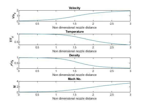
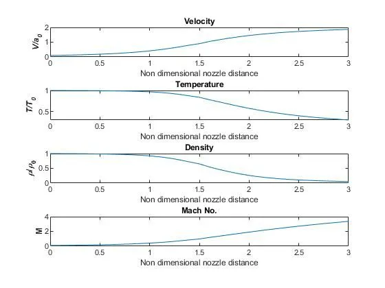
The steady-state distribution of primitive variables inside the nozzle:
The steady-state distribution of primitive variables shows how the variables change along the span of the nozzle from the convergent part to the divergent part for non-conservative and conservative forms of
the governing equations.
Non-Conservative Form:
Conservative Form:
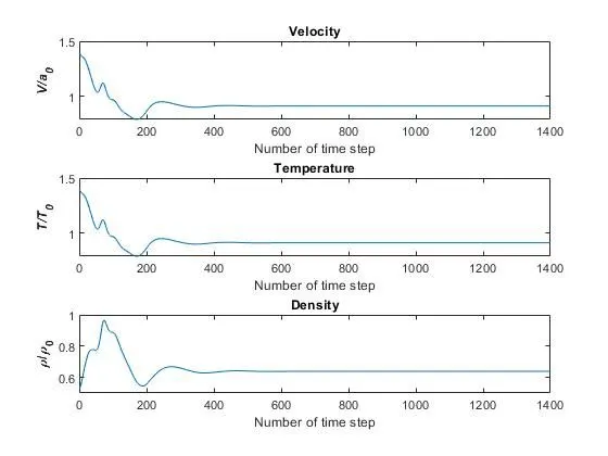
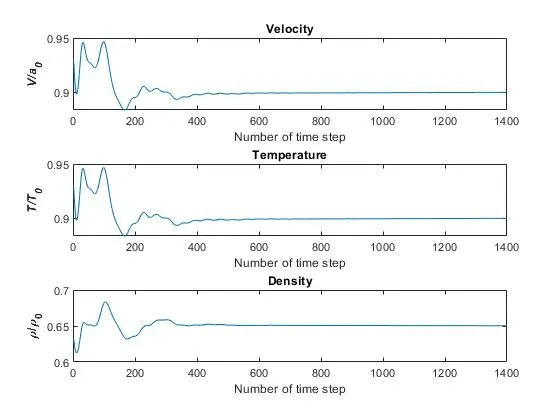
Time-wise variation of the primitive variables:
The time-wise variation of the primitive variables from the initial condition to the 1400 time step is shown in the figures. It can be seen that the variation is maximum in early timesteps for both cases. But in comparison, in the nonconservative form, these die down around the 300th timestep while for the conservative form the changes are prominent around 400th-time
step.
Non-Conservative Form:
Conservative Form:
Variation of Mass flow rate distribution inside the nozzle at different time steps during the time-marching process:
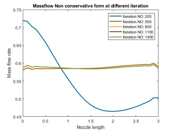
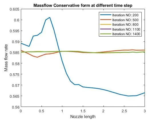
Here the non-dimensional mass flow is plotted as the function of the non-dimensional distance through the nozzle. Five different curves are
shown. Initially, the curves show huge variation and as time passes the variation is diminished and finally comes to a constant value.
Comparison of Normalized mass flow rate distributions of both forms:
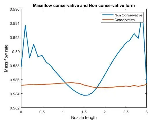
Now, we compare the steady-state variations of the mass flow obtained with the non-conservative and conservative Steady-state variation of the conservative form was compared to that of the non-conservative form. Here we can see that the conservative form has a satisfactory value compared to the value obtained from the non-conservative form. in conservation form preserving the mass throughout the flowfield as it is a dependent variable in the equation. But in non-conservation form, the dependent variables are primary flow variables and mass flow is obtained as a secondary result. The steady-state mass flow results obtained with the conservation form are hence closer to the exact analytical value of 0.549.
The grid independence test
| `frac{rho^ast} {rho_0^ast}` |
`frac{T^ast} {T_0^ast}` |
Mach Number M |
|
| Exact analytical solution |
0.634 | 0.833 | 1.000 |
| Conservation form, numerical results (31 points) |
0.650 | 0.840 | 0.981 |
| Non-Conservation form, numerical results (31 points) |
0.721 | 0.836 | 0.999 |
| Nonconservation form, numerical results (61 points) |
0.637 | 0.835 | 0.999 |
| Conservation form, numerical results (61 points) |
0.638 | 0.835 | 0.991 |
Conclusions
The conservative form gives a better mass flow distribution compared to the non-conservative form