Week 1- Mixing Tee
Aim:
i) To set up steady-state simulations to compare the mixing effectiveness when hot inlet temperature is 360C & the Cold inlet is at 190C.
- Case i:
- Short mixing tee with a hot inlet velocity of 3m/s.
- Momentum ratio of 2, 4.
- Case ii:
- Long mixing tee with a hot inlet velocity of 3m/s.
- Momentum ratio of 2, 4.
ii) To carry out a mesh independance study to find the dependednce of mesh and output result in any one of the above mentioned case.
Numerical results:
`T_{mixture} = (m_{hot}*T_{hot}+m_{cold}*T_{cold})/(m_{hot}+m_{cold})`
`T_{mixture}` = Temperature of the mixture in `.^oC`
`m_{hot}` = mass of hot air. = `rho*A_{hot}*V_{hot}`
`m_{cold}` = mass of cold air. = `rho*A_{cold}*V_{cold}`
`T_{hot}` = Temperature of hot air. = `36^oC`
`T_{cold}` = Temperature of cold air. = `19^oC`.
`T_{mixture}` = `(1.2*0.0009*36+1.2*0.0002*19)/(1.2*0.0009+1.2*0.0002)` = `30.76^oC`
Pre-Processing:
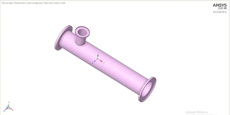
Case I
Raw model:
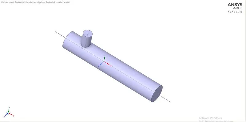
Volume extracted:
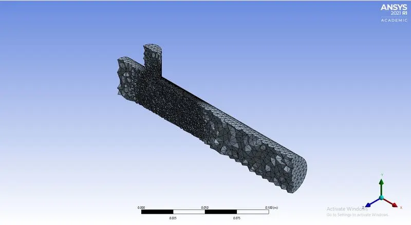
Sectional view of meshed model:
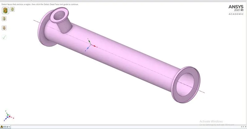
Case II
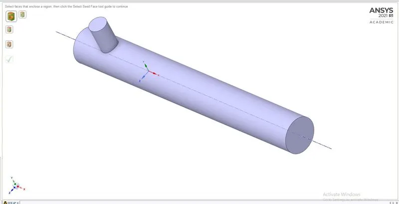
Raw model:
Volume extracted:
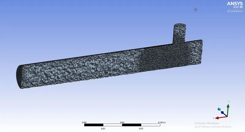
Sectional view of meshed model:
- The STP file of the model was initially imported to the spaceclaim
- By using volume extract from the prepeare menu the volume through which the fluid dlows is extracted and the rest of the TEE was suppressed for physics
- Now the extracted volume is meshed and the simulation was ran for a trial now the mixing length of two streams was captured and now again returnd to meshing and we introduce a sizing method in which we selelct type as 'sphere of influence' and we refine the mesh inside radius of the sphere.
- we refine the elements inside the sphere to capture the mixing region perfectly.
Results:
- The simulation was run in steady state condition
- k-epsilon realisable model was mainly used for solving all the cases as the K-omega model took more computational power and time for converging when compared to the k-epsilon model for same momentum ratio and elemental size. Since K-omega is mainly used for capturing the variation near to the wall.
- Working fluid was slelcted as air
- Now we define the inlet velocity and temperature of fluids in each inlets (hot and cold).
- Now under the results we define the reports for avg temp and standered deviation.
- We initialze with hybrid initialization and run for a specified no. of iterations.
Post-Processing:
Case I
Momentum Ratio: 2
Convergance plot:
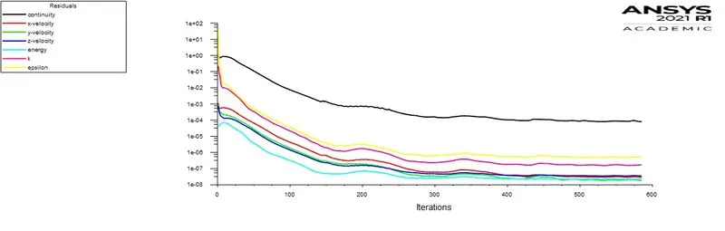
Turbulence model: K-epsilon REALIZABLE
Velocity of hot inlet: 3m/s
Velocity of cold inlet: 6m/s
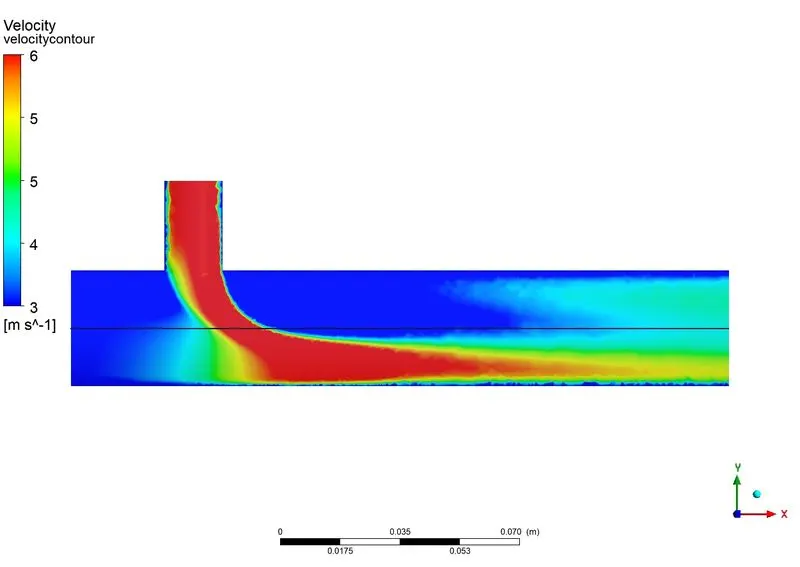
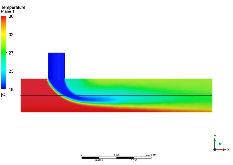
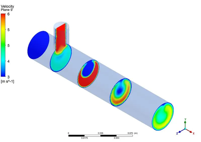
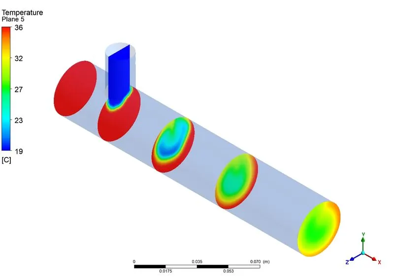
Contour Plots:
- Velocity (along the pipe)
- Temperature (along the pipe)
- Velocity (accross the pipe)
- Temperature(accross the pipe)
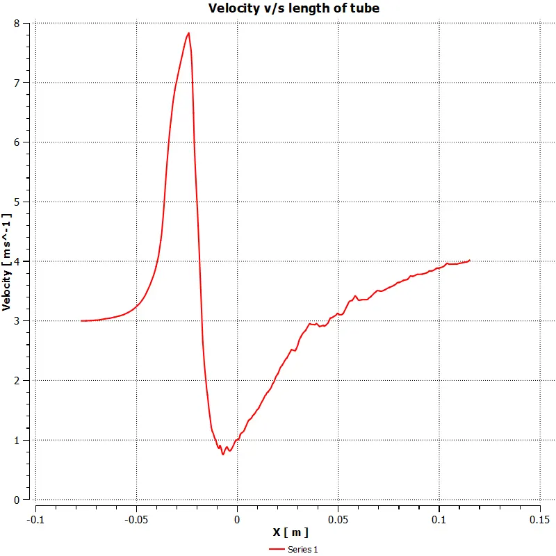
Line Plots:
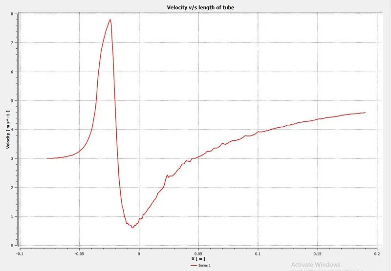
- Velocity (along the pipe)
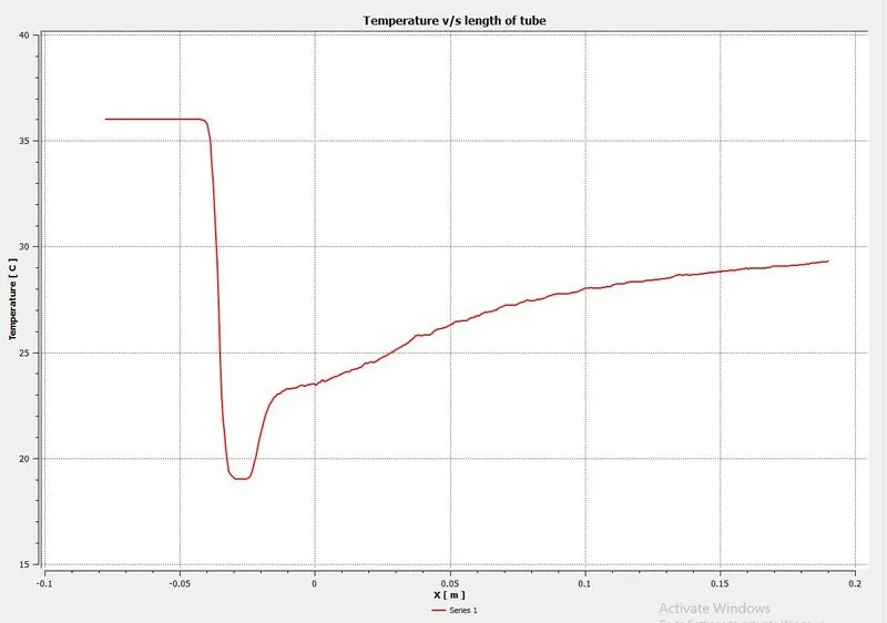
- Temperature (along
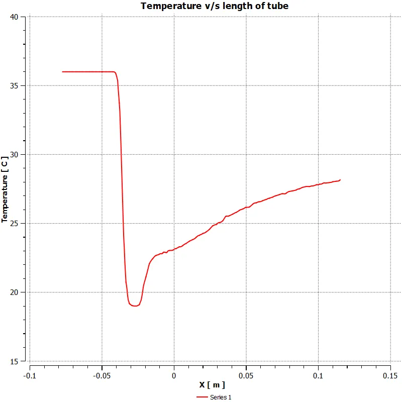 the pipe)
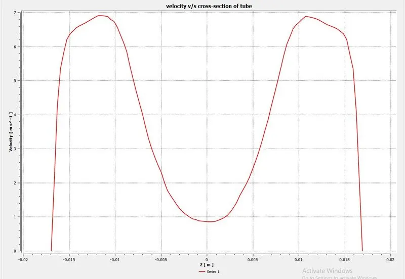
- Velocity (accross the pipe)
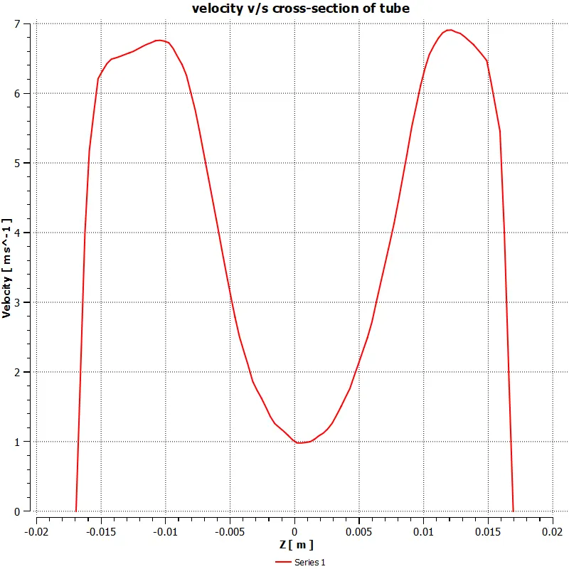
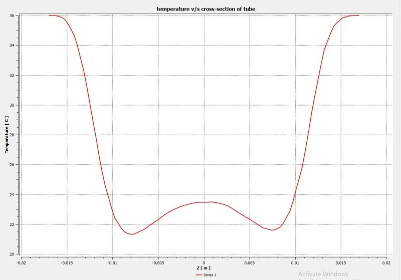
- Temperature(accross the pipe)
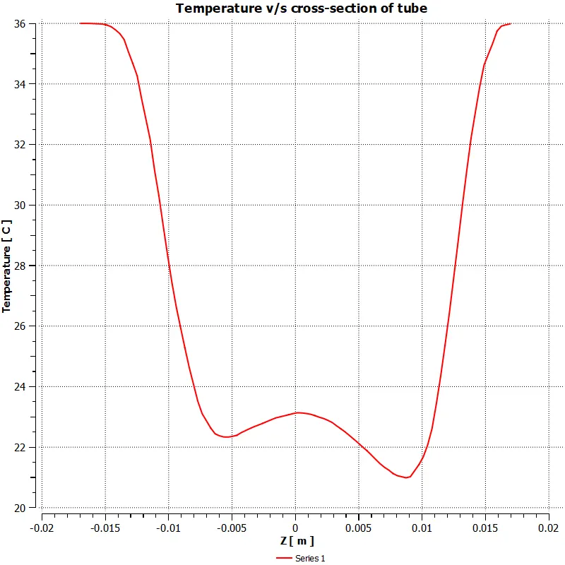
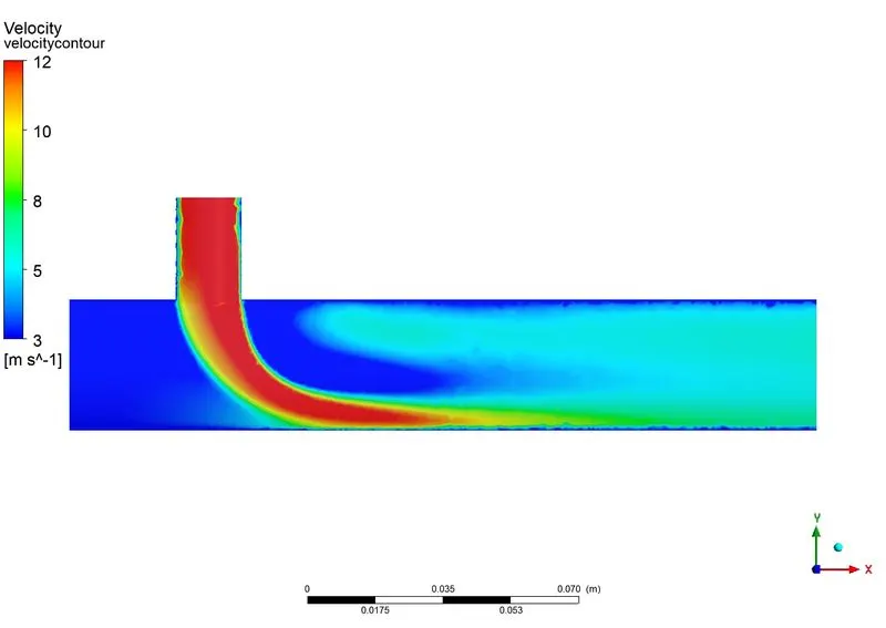
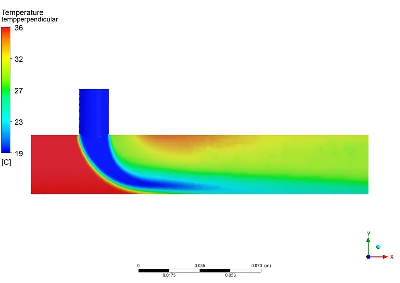
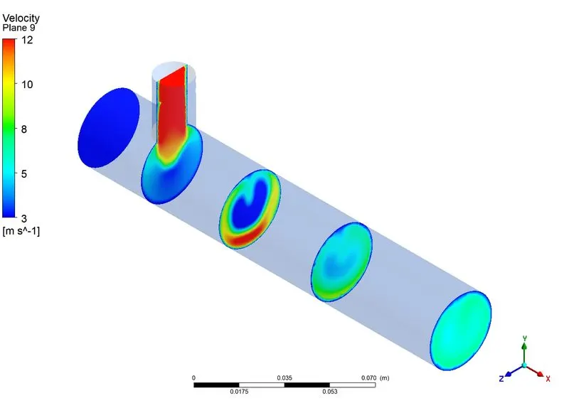
Momentum Ratio: 4
Convergance plot:
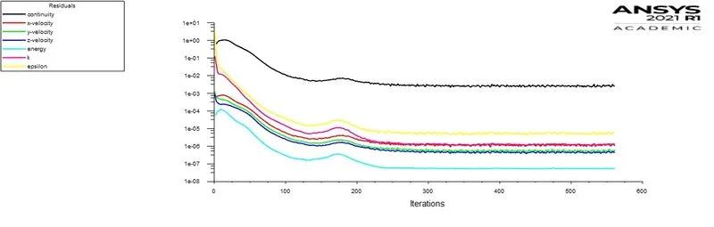
Turbulence model: K-epsilon REALIZABLE
Velocity of hot inlet: 3m/s
Velocity of cold inlet: 12m/s
Contour Plots:
- Velocity (along the pipe)
- Temperature (along the pipe)
- Velocity (accross the pipe)
- Temperature(accross the pipe)
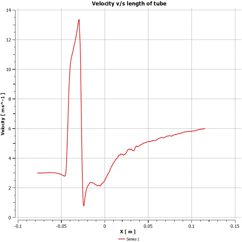
Line Plots:
- Velocity (along the pipe)
- Temperature (along the pipe)
- Velocity (accross the pipe)
- Temperature(accross the pipe)
Case II
Momentum Ratio: 2
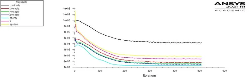
Convergance plot:
Turbulence model: K-epsilon REALIZABLE
Velocity of hot inlet: 3m/s
Velocity of cold inlet: 6m/s
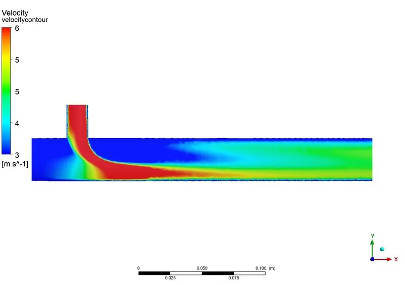
Contour Plots:
- Velocity (along the pipe)
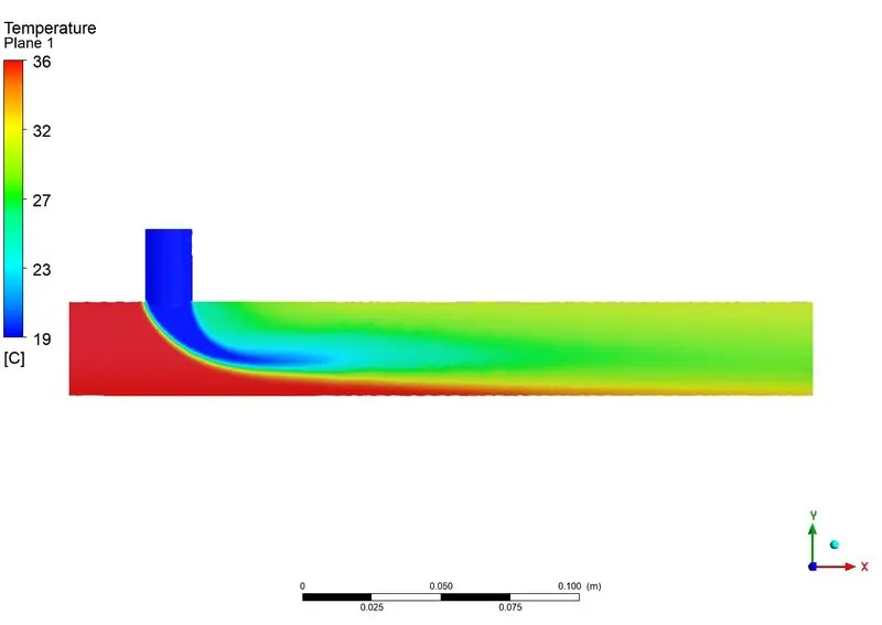
- Temperature (along the pipe)
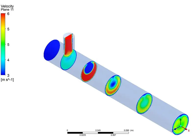
- Velocity (accross the pipe)
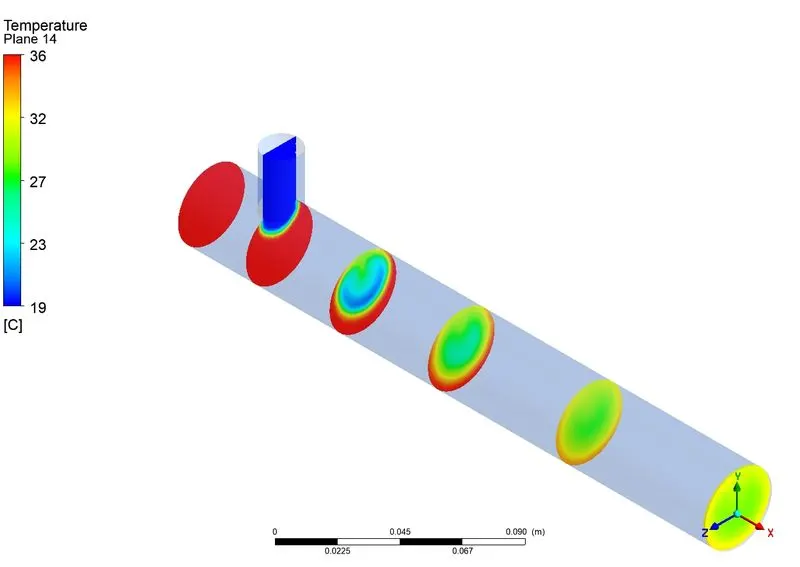
- Temperature(accross the pipe)
Line Plots:
- Velocity (along the pipe)
- Temperature (along the pipe)
- Velocity (accross the pipe)
- Temperature(accross the pipe)
Momentum Ratio: 4
Convergance plot:
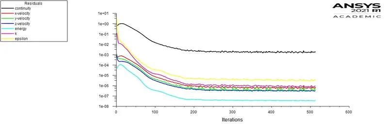
Turbulence model: k-epsilon REALIZABLE
Velocity of hot inlet: 3m/s
Velocity of cold inlet: 12m/s
Contour Plots:
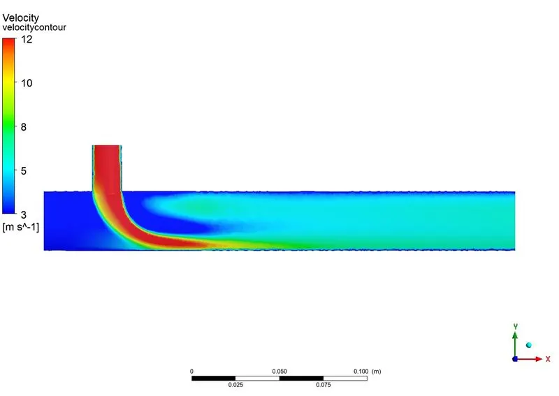
- Velocity (along the pipe)
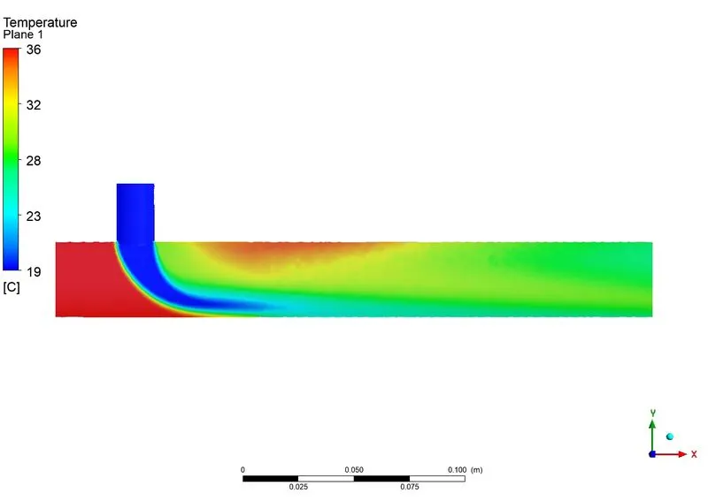
- Temperature (along the pipe)
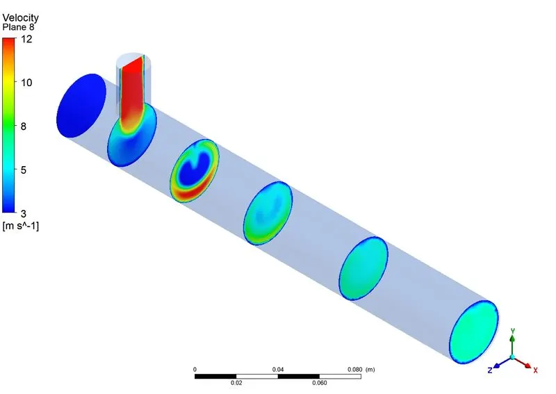
- Velocity (accross the pipe)
- Temperature(accross the pipe)
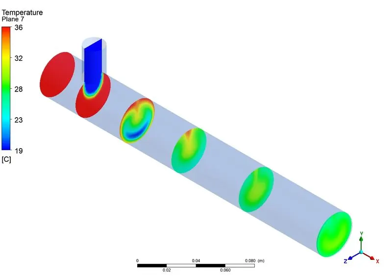
Line Plots:
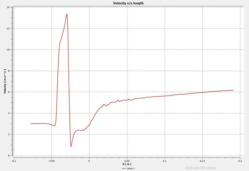
- Velocity (along the pipe)
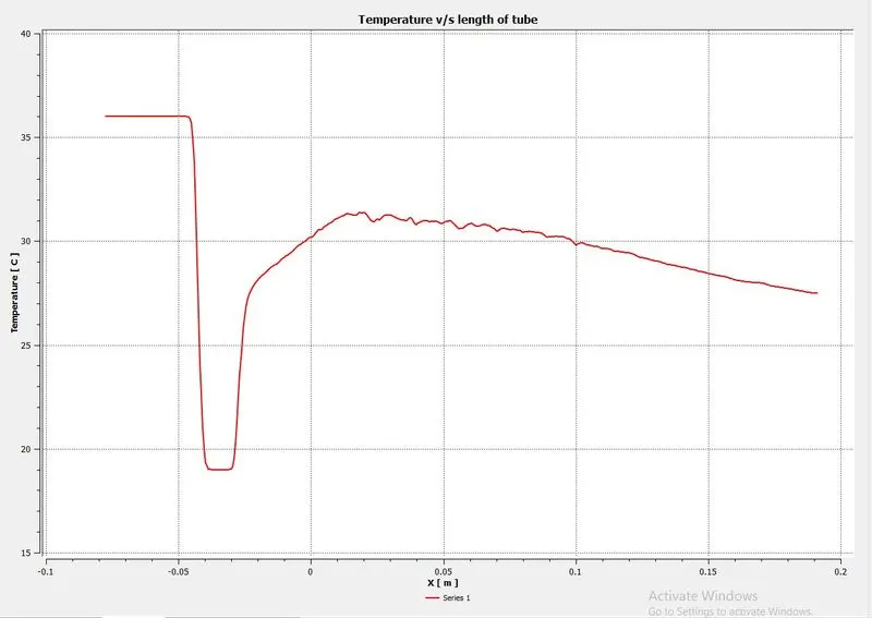
- Temperature (along the pipe)
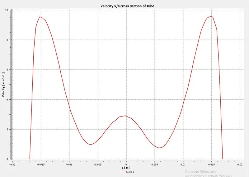
- Velocity (accross the pipe)
- Temperature(accross the pipe)
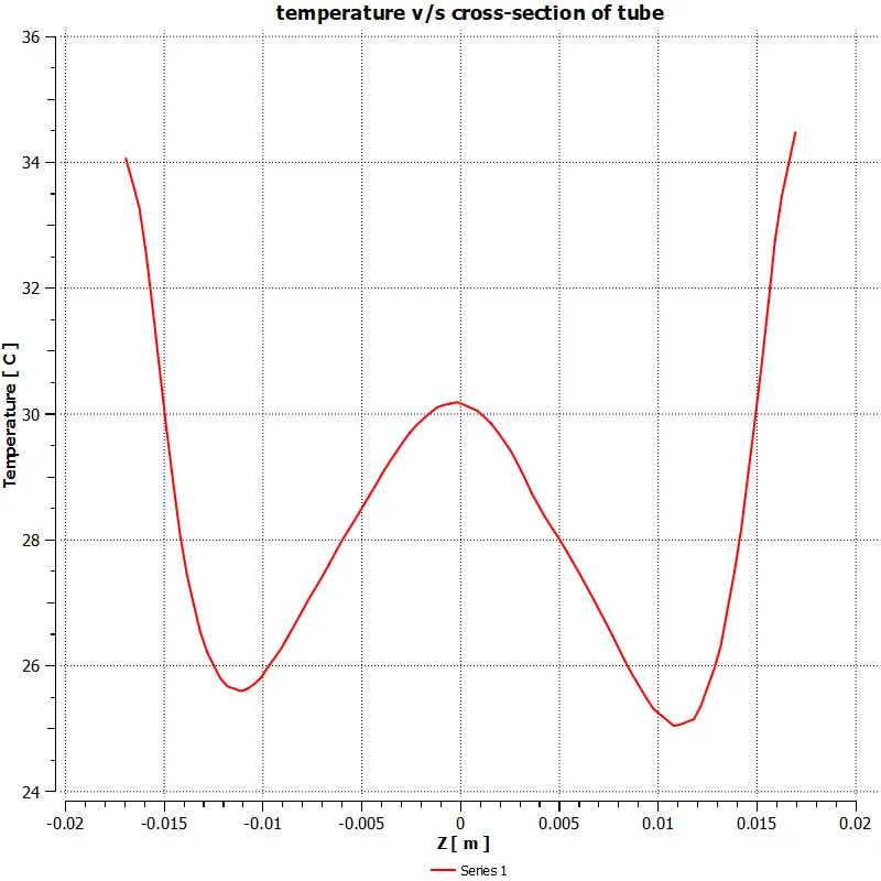
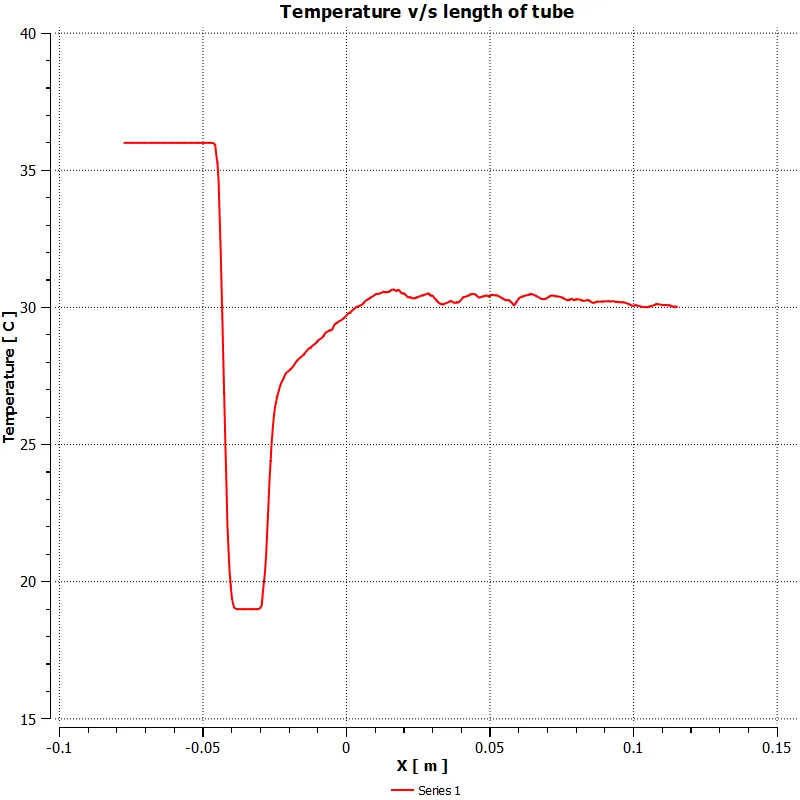
- From the results of the graph it can be seen that as fluid flows along the length at mixing region the velocity spikes to a near value of the cold inlet velocity and starts to avg as it reaches the outlet.
- Same with the case of temperature as the fluid flows at the region of mixing the temperature drops to a near low value of the cold fluid temperature and as it moves to outlet it averages due to process of mixing.
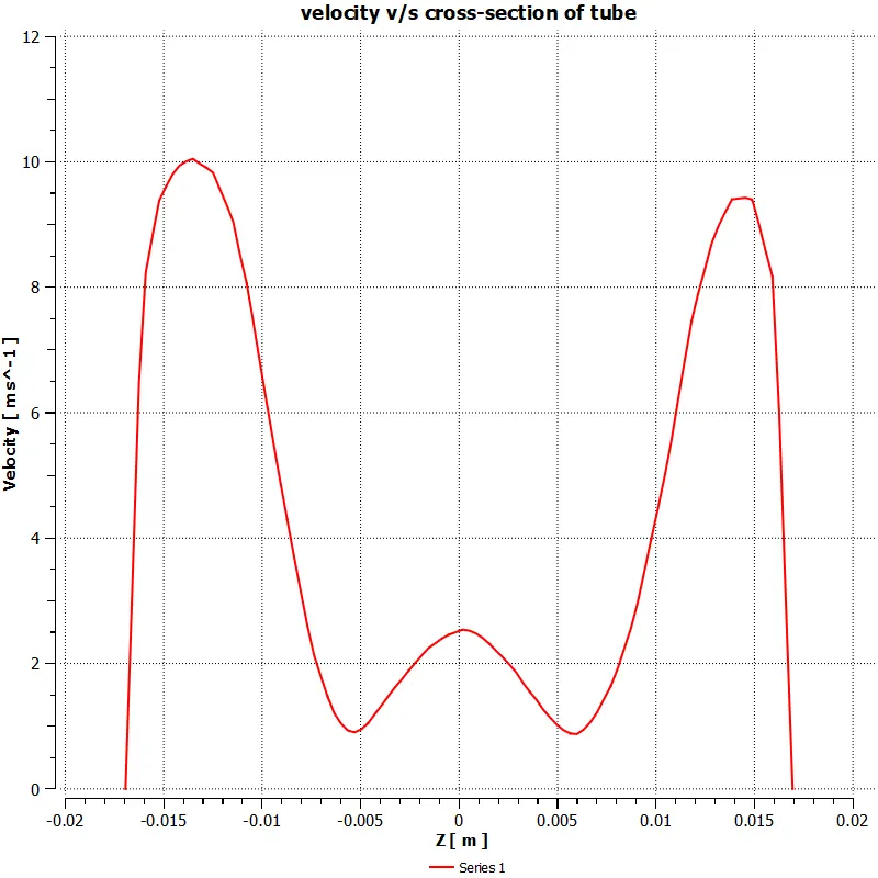
- the variation of temperature accross the walls show that since walll being at no slip condition the velocity is zero near the wall and as it moves to the centre the velocity increases and since the region selected is just after the mixing region,
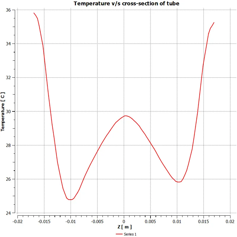
- Due to the process of mixing the outer fluid wraps the cold fluid and this being the reason for higher temperature at outside and the temperature drops as we move to centre.
Comparison of cell count avg outlet temp and number of iteration to converge:
| Momentum Ratio | Avg outlet temperature | Cell Count |
Number of iteration to converge
|
|
| Case 1 | 2 | 30.31 | 465855 | 400 |
| Case 1 | 4 | 27.56 | 465855 | 300 |
| Case 2 | 2 | 30.41 | 500739 | 300 |
| Case 2 | 4 | 27.49 | 500739 | 300 |
- From the comparison shown below it is of the view that the length of the TEE has a very less oralmost no effect on the average outlet temperature. but depend upon the inlet velocity of the cold air.
- It is thus advisable to use a short TEE as the cell count is comparitively low owing to less computation time and power.
Mesh independednt study on case I (Momentum ratio:2)
| Elemental Size(mm) | No. Of Elements |
Avg outlet temperature
|
| 4 | 415722 | 30.26 |
| 3 | 426268 | 30.27 |
| 2 | 465855 | 30.31 |
| 1.7 | 499051 | 30.31 |
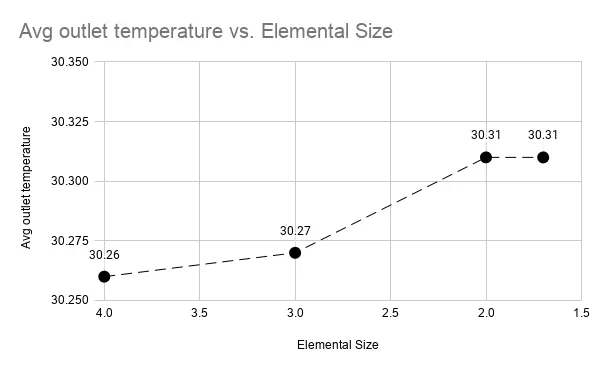
- From the mesh independent study carried out it can be seen that on reducing the element size the avg outlet temperature is found to increase till a parrticular value (ie: 2mm) and after that it is found to be almost constant with almost zero change.
- Thus it can be inferred that the outlet temperature is found to be independent of the mesh size.
Conclusion:
- From the results of the temperature plots it can be clearly interpretted that in increasing the inlet velocity the mixing is found to increase owing to a decrease in the avg outlet temperature. This is clear from the results of increasing momentum ratio.
- thus on increasing the momentum ratio the avg outlet temperature is found to decrease.
- The length of the TEE has zero or negligible effect on the avg outlet temperature this is clear from the case1 and 2 for same momentum ratio the avg outlet temp is found to be almost same with negligible change only.